Introduction to R
24 minute read
Overview
What is R?
R is a powerful statistical environment and programming language for the analysis and visualization of data. The associated Bioconductor and CRAN package repositories provide many additional R packages for statistical data analysis for a wide array of research areas. The R software is free and runs on all common operating systems.
Why Using R?
- Complete statistical environment and programming language
- Efficient functions and data structures for data analysis
- Powerful graphics
- Access to fast growing number of analysis packages
- Most widely used language in bioinformatics
- Is standard for data mining and biostatistical analysis
- Technical advantages: free, open-source, available for all OSs
Books and Documentation
- simpleR - Using R for Introductory Statistics (John Verzani, 2004) - URL
- Bioinformatics and Computational Biology Solutions Using R and Bioconductor (Gentleman et al., 2005) - URL
- More on this see “Finding Help” section in UCR Manual - URL
R Working Environments

R Projects and Interfaces
Some R working environments with support for syntax highlighting and utilities to send code to the R console:
- RStudio/Posit Desktop: excellent choice for beginners (Cheat Sheets)
- RStudio/Posit Server: web-based UI for RStudio. Available at UCR via onDemand (old standalone web instance will be discontinued).
- RStudio/Posit Cloud: cloud-based RStudio Server
- Vim-R-Tmux: R working environment based on vim and tmux.
- Emacs (ESS add-on package)
- gedit, Rgedit, RKWard, Eclipse, Tinn-R, Notepad++, NppToR
Example: RStudio
New integrated development environment (IDE) for R. Highly functional for both beginners and advanced.

RStudio IDE
Some userful shortcuts: Ctrl+Enter (send code), Ctrl+Shift+C (comment/uncomment), Ctrl+1/2 (switch window focus)
Example: Nvim-R-Tmux
Terminal-based Working Environment for R: Nvim-R-Tmux.

Nvim-R-Tmux IDE for R
Install and usage instructions for Nvim-R are provided in this slide show and this tutorial. The most detailed instructions can be found on the Nvim-R_Tmux GitHub repos.
R Package Repositories
- CRAN (>14,000 packages) general data analysis - URL
- Bioconductor (>2,000 packages) bioscience data analysis - URL
- Omegahat (>90 packages) programming interfaces - URL
- RStudio packages - URL
Working routine for tutorials
When working in R, a good practice is to write all commands directly into an R script, instead of the R console, and then send the commands for execution to the R console with the Ctrl+Enter shortcut in RStudio/Posit, or similar shortcuts in other R coding environments, such as Nvim-R. This way all work is preserved and can be reused in the future.
The following instructions in this section provide a short overview of the standard working routine users should use to load R-based tutorials of this website into an R IDE (Nvim-R or RStudio). For Nvim-R on HPCC users can visit the Quick Demo slide here.
-
Download
*.Rmdor*.Rfile. These so called source files are always linked on the top right corner of each tutorial. The ones for this tutorial are here. The file download can be accomplished viadownload.filefrom within R (see below),wgetfrom the command-line or with the save function in a user’s web browser. The following downloads theRmdfile of this tutorial viadownload.filefrom the R console.download.file("https://raw.githubusercontent.com/tgirke/GEN242//main/content/en/tutorials/rbasics/Rbasics.Rmd", "Rbasics.Rmd") -
Load
*.Rmdor*.Rfile in Neovim (Nvim-R) or RStudio. -
Send code from code editor to R console by pushing
space barin Neovim (Nvim-R) orCtrl + Enterin RStudio. In*.Rmdfiles the code lines are in so called code chunks and only those ones can be sent to the console. To obtain in Neovim a connected R session one has to initiate by pressing the\rfkey combination. For details see here.
Installation of R, RStudio and R Packages
-
Install R for your operating system from CRAN.
-
Install RStudio from RStudio.
-
Install CRAN Packages from R console like this:
install.packages(c("pkg1", "pkg2")) install.packages("pkg.zip", repos=NULL) -
Install Bioconductor packages as follows:
if (!requireNamespace("BiocManager", quietly = TRUE)) install.packages("BiocManager") # Installs BiocManager if not available yet BiocManager::version() # Reports Bioconductor version BiocManager::install(c("pkg1", "pkg2")) # Installs packages specified under "pkg1" -
For more details consult the Bioc Install page and BiocManager package.
-
Instructions for upgrading R and packages to newer versions are given at the end of this tutorial here.
Getting Around
Startup and Closing Behavior
-
Starting R: The R GUI versions, including RStudio, under Windows and Mac OS X can be opened by double-clicking their icons. Alternatively, one can start it by typing
Rin a terminal (default under Linux). -
Startup/Closing Behavior: The R environment is controlled by hidden files in the startup directory:
.RData,.Rhistoryand.Rprofile(optional). -
Closing R:
q()
Save workspace image? [y/n/c]:
- Note:
When responding with
y, then the entire R workspace will be written to the.RDatafile which can become very large. Often it is better to selectnhere, because a much better working pratice is to save an analysis protocol to anRorRmdsource file. This way one can quickly regenerate all data sets and objects needed in a future session.
Navigating directories
List objects in current R session
ls()
Return content of current working directory
dir()
Return path of current working directory
getwd()
Change current working directory
setwd("/home/user")
Checking information about files (collection of useful commands)
list.files(path="./", pattern="*.txt$", full.names=TRUE) # lists files in directory
file.exists(c("file1", "file2")) # check if provided files exist
file.size(list.files(path="./", pattern=".txt$", full.names=TRUE)) # return file sizes
file.info(list.files(path="./", pattern=".txt$", full.names=TRUE)) # retrive detailed information about files
Basic Syntax
Create an object with the assignment operator <- or =
object <- ...
General R command syntax
object <- function_name(arguments)
object <- object[arguments]
Instead of the assignment operator one can use the assign function
assign("x", function(arguments))
To simplify chaining of serveral operations, dplyr (magrittr) provides the %>% (pipe) operator,
where x %>% f(y) turns into f(x, y). This way one can pipe together multiple
operations by writing them from left-to-right or top-to-bottom. This makes for
easy to type and readable code. Details on this are provided in the dplyr tutorial here.
... %>% ...
Finding help
?function_name
Load one or more R packages (libraries)
library("my_library") # Single package
lapply(c("my_library1", "my_library2"), require, character.only = TRUE) # Multiple packages
List functions defined by a library
library(help="my_library")
Load library manual (PDF or HTML file)
vignette("my_library")
Execute an R script from within R
source("my_script.R")
Execute an R script from command-line (the first of the three options is preferred)
$ Rscript my_script.R
$ R CMD BATCH my_script.R
$ R --slave < my_script.R
Data Types
Numeric data
Example: 1, 2, 3, ...
x <- c(1, 2, 3)
x
## [1] 1 2 3
is.numeric(x)
## [1] TRUE
as.character(x)
## [1] "1" "2" "3"
Character data
Example: "a", "b", "c", ...
x <- c("1", "2", "3")
x
## [1] "1" "2" "3"
is.character(x)
## [1] TRUE
as.numeric(x)
## [1] 1 2 3
Complex data
Example: mix of both
c(1, "b", 3)
## [1] "1" "b" "3"
Logical data
Example: TRUE of FALSE
x <- 1:10 < 5
x
## [1] TRUE TRUE TRUE TRUE FALSE FALSE FALSE FALSE FALSE FALSE
!x
## [1] FALSE FALSE FALSE FALSE TRUE TRUE TRUE TRUE TRUE TRUE
which(x) # Returns index for the 'TRUE' values in logical vector
## [1] 1 2 3 4
Data Objects
Object types
- List of common object types
vectors: ordered collection of numeric, character, complex and logical values.factors: special type vectors with grouping information of its componentsdata.framesincluding modern variantsDataFrame,tibbles, etc.: two dimensional structures with different data typesmatrices: two dimensional structures with data of same typearrays: multidimensional arrays of vectorslists: general form of vectors with different types of elementsfunctions: piece of code- Many more …
- Simple rules for naming objects and their components
- Object, row and column names should not start with a number
- Avoid spaces in object, row and column names
- Avoid special characters like ‘#’
Vectors (1D)
Definition: numeric or character
myVec <- 1:10; names(myVec) <- letters[1:10]
myVec <- setNames(1:10, letters[1:10]) # Same as above in single step
myVec[1:5]
## a b c d e
## 1 2 3 4 5
myVec[c(2,4,6,8)]
## b d f h
## 2 4 6 8
myVec[c("b", "d", "f")]
## b d f
## 2 4 6
Factors (1D)
Definition: vectors with grouping information
factor(c("dog", "cat", "mouse", "dog", "dog", "cat"))
## [1] dog   cat   mouse dog   dog   cat
## Levels: cat dog mouse
Matrices (2D)
Definition: two dimensional structures with data of same type
myMA <- matrix(1:30, 3, 10, byrow = TRUE)
class(myMA)
## [1] "matrix" "array"
myMA[1:2,]
##      [,1] [,2] [,3] [,4] [,5] [,6] [,7] [,8] [,9] [,10]
## [1,]    1    2    3    4    5    6    7    8    9    10
## [2,]   11   12   13   14   15   16   17   18   19    20
myMA[1, , drop=FALSE]
##      [,1] [,2] [,3] [,4] [,5] [,6] [,7] [,8] [,9] [,10]
## [1,]    1    2    3    4    5    6    7    8    9    10
class(as.data.frame(myMA)) # convert matrix to data.frame
## [1] "data.frame"
Data Frames (2D)
Definition: data.frames are two dimensional objects with data of variable types
myDF <- data.frame(Col1=1:10, Col2=10:1)
myDF[1:2, ]
##   Col1 Col2
## 1    1   10
## 2    2    9
class(as.matrix(myDF)) # convert data.frame to matrix
## [1] "matrix" "array"
Tibbles
Tibbles are a more modern version of data.frames. Among many other advantages, one can see
here that tibbles have a nicer printing bahavior. Much more detailed information on this object
class is provided in the dplyr/tidyverse manual section.
library(tidyverse)
as_tibble(iris)
## # A tibble: 150 × 5
##    Sepal.Length Sepal.Width Petal.Length Petal.Width Species
##           <dbl>       <dbl>        <dbl>       <dbl> <fct>
##  1          5.1         3.5          1.4         0.2 setosa
##  2          4.9         3            1.4         0.2 setosa
##  3          4.7         3.2          1.3         0.2 setosa
##  4          4.6         3.1          1.5         0.2 setosa
##  5          5           3.6          1.4         0.2 setosa
##  6          5.4         3.9          1.7         0.4 setosa
##  7          4.6         3.4          1.4         0.3 setosa
##  8          5           3.4          1.5         0.2 setosa
##  9          4.4         2.9          1.4         0.2 setosa
## 10          4.9         3.1          1.5         0.1 setosa
## # … with 140 more rows
Note: The above example uses the iris test dataset that is available in every R installation without explicitly importing or loading it. The following examples will often make use of this dataset.
Arrays
Definition: data structure with one, two or more dimensions
Lists
Definition: containers for any object type
myL <- list(name="Fred", wife="Mary", no.children=3, child.ages=c(4,7,9))
myL
## $name
## [1] "Fred"
##
## $wife
## [1] "Mary"
##
## $no.children
## [1] 3
##
## $child.ages
## [1] 4 7 9
myL[[4]][1:2]
## [1] 4 7
Functions
Definition: piece of code
myfct <- function(arg1, arg2, ...) {
	function_body
}
Subsetting of data objects
(1.) Subsetting by positive or negative index/position numbers
myVec <- 1:26; names(myVec) <- LETTERS
myVec[1:4]
## A B C D
## 1 2 3 4
(2.) Subsetting by same length logical vectors
myLog <- myVec > 10
myVec[myLog]
##  K  L  M  N  O  P  Q  R  S  T  U  V  W  X  Y  Z
## 11 12 13 14 15 16 17 18 19 20 21 22 23 24 25 26
(3.) Subsetting by field names
myVec[c("B", "K", "M")]
##  B  K  M
##  2 11 13
(4.) Subset with $ sign: references a single column or list component by its name
iris$Species[1:8]
## [1] setosa setosa setosa setosa setosa setosa setosa setosa
## Levels: setosa versicolor virginica
Important Utilities
Combining Objects
The c function combines vectors and lists
c(1, 2, 3)
## [1] 1 2 3
x <- 1:3; y <- 101:103
c(x, y)
## [1] 1 2 3 101 102 103
The cbind and rbind functions can be used to append columns and rows, respecively.
ma <- cbind(x, y)
ma
##      x   y
## [1,] 1 101
## [2,] 2 102
## [3,] 3 103
rbind(ma, ma)
##      x   y
## [1,] 1 101
## [2,] 2 102
## [3,] 3 103
## [4,] 1 101
## [5,] 2 102
## [6,] 3 103
Accessing Dimensions of Objects
Length and dimension information of objects
length(iris$Species)
## [1] 150
dim(iris)
## [1] 150 5
Accessing Name Slots of Objects
Accessing row and column names of 2D objects
rownames(iris)[1:8]
## [1] "1" "2" "3" "4" "5" "6" "7" "8"
colnames(iris)
## [1] "Sepal.Length" "Sepal.Width" "Petal.Length" "Petal.Width" "Species"
Return name field of vectors and lists
names(myVec)
##  [1] "A" "B" "C" "D" "E" "F" "G" "H" "I" "J" "K" "L" "M" "N" "O" "P" "Q" "R" "S" "T" "U" "V" "W" "X"
## [25] "Y" "Z"
names(myL)
## [1] "name" "wife" "no.children" "child.ages"
Sorting Objects
The function sort returns a vector in ascending or descending order.
sort(10:1)
## [1] 1 2 3 4 5 6 7 8 9 10
The function order returns a sorting index for sorting an object alphanumerically.
sortindex <- order(iris[,1], decreasing = FALSE)
sortindex[1:12]
## [1] 14 9 39 43 42 4 7 23 48 3 30 12
iris[sortindex,][1:2,]
##    Sepal.Length Sepal.Width Petal.Length Petal.Width Species
## 14          4.3         3.0          1.1         0.1  setosa
## 9           4.4         2.9          1.4         0.2  setosa
sortindex <- order(-iris[,1]) # Same as decreasing=TRUE
Sorting multiple columns
iris[order(iris$Sepal.Length, iris$Sepal.Width),][1:2,]
##    Sepal.Length Sepal.Width Petal.Length Petal.Width Species
## 14          4.3         3.0          1.1         0.1  setosa
## 9           4.4         2.9          1.4         0.2  setosa
Check differences
To check whether the values in two objects are the same, one can use the == comparison operator.
The all function allows to find out whether all values are the same. To check whether two objects
are exactly identical, use the identical function.
myma <- iris[1:2,]
myma == iris[1:2,]
##   Sepal.Length Sepal.Width Petal.Length Petal.Width Species
## 1         TRUE        TRUE         TRUE        TRUE    TRUE
## 2         TRUE        TRUE         TRUE        TRUE    TRUE
all(myma == iris[1:2,])
## [1] TRUE
myma[1,1] <- 1 # changes value in first cell
all(myma == iris[1:2,])
## [1] FALSE
Operators and Calculations
Comparison Operators
Comparison operators: ==, !=, <, >, <=, >=
1==1
## [1] TRUE
Logical operators for boolean operations: AND: &, OR: |, NOT: !
x <- 1:10; y <- 10:1
x > y & x > 5
## [1] FALSE FALSE FALSE FALSE FALSE TRUE TRUE TRUE TRUE TRUE
Basic Calculations
To look up math functions, see Function Index here
x + y
## [1] 11 11 11 11 11 11 11 11 11 11
sum(x)
## [1] 55
mean(x)
## [1] 5.5
apply(iris[1:6,1:3], 1, mean)
##        1        2        3        4        5        6
## 3.333333 3.100000 3.066667 3.066667 3.333333 3.666667
Reading and Writing External Data
Import of tabular data
Import of a tab-delimited tabular file
myDF <- read.delim("myData.xls", sep="\t")
Import of Google Sheets. The following example imports a sample Google Sheet from here.
Detailed instructions for interacting from R with Google Sheets with the required googlesheets4 package are here.
library(googlesheets4)
gs4_deauth() # Easiest method for reading public access sheets
mysheet <- read_sheet("1U-32UcwZP1k3saKeaH1mbvEAOfZRdNHNkWK2GI1rpPM", skip=4)
myDF <- as.data.frame(mysheet)
myDF
Import from Excel sheets works well with readxl. For details see the readxl package manual here. Note: working with tab- or comma-delimited files is more flexible and highly preferred for automated analysis workflows.
library("readxl")
mysheet <- read_excel(targets_path, sheet="Sheet1")
Additional import functions are described in the readr package section here.
Export of tabular data
write.table(myDF, file="myfile.xls", sep="\t", quote=FALSE, col.names=NA)
Line-wise import
myDF <- readLines("myData.txt")
Line-wise export
writeLines(month.name, "myData.txt")
Export R object
mylist <- list(C1=iris[,1], C2=iris[,2]) # Example to export
saveRDS(mylist, "mylist.rds")
Import R object
mylist <- readRDS("mylist.rds")
Copy and paste into R
On Windows/Linux systems
read.delim("clipboard")
On Mac OS X systems
read.delim(pipe("pbpaste"))
Copy and paste from R
On Windows/Linux systems
write.table(iris, "clipboard", sep="\t", col.names=NA, quote=FALSE)
On Mac OS X systems
zz <- pipe('pbcopy', 'w')
write.table(iris, zz, sep="\t", col.names=NA, quote=FALSE)
close(zz)
Homework 3A
Homework 3A: Object Subsetting Routines and Import/Export
Useful R Functions
Unique entries
Make vector entries unique with unique
length(iris$Sepal.Length)
## [1] 150
length(unique(iris$Sepal.Length))
## [1] 35
Count occurrences
Count occurrences of entries with table
table(iris$Species)
##
##     setosa versicolor  virginica
##         50         50         50
Aggregate data
Compute aggregate statistics with aggregate
aggregate(iris[,1:4], by=list(iris$Species), FUN=mean, na.rm=TRUE)
##      Group.1 Sepal.Length Sepal.Width Petal.Length Petal.Width
## 1     setosa        5.006       3.428        1.462       0.246
## 2 versicolor        5.936       2.770        4.260       1.326
## 3  virginica        6.588       2.974        5.552       2.026
Intersect data
Compute intersect between two vectors with %in%
month.name %in% c("May", "July")
## [1] FALSE FALSE FALSE FALSE TRUE FALSE TRUE FALSE FALSE FALSE FALSE FALSE
Merge data frames
Join two data frames by common field entries with merge (here row names by.x=0). To obtain only the common rows, change all=TRUE to all=FALSE. To merge on specific columns, refer to them by their position numbers or their column names.
frame1 <- iris[sample(1:length(iris[,1]), 30), ]
frame1[1:2,]
##     Sepal.Length Sepal.Width Petal.Length Petal.Width   Species
## 147          6.3         2.5          5.0         1.9 virginica
## 49           5.3         3.7          1.5         0.2    setosa
dim(frame1)
## [1] 30 5
my_result <- merge(frame1, iris, by.x = 0, by.y = 0, all = TRUE)
dim(my_result)
## [1] 150 11
Graphics in R
Advantages
- Powerful environment for visualizing scientific data
- Integrated graphics and statistics infrastructure
- Publication quality graphics
- Fully programmable
- Highly reproducible
- Full LaTeX and Markdown support via
knitrandR markdown - Vast number of R packages with graphics utilities
Documentation for R Graphics
General
- Graphics Task Page - URL
- R Graph Gallery - URL
- R Graphical Manual - URL
- Paul Murrell’s book R (Grid) Graphics - URL
Interactive graphics
Graphics Environments
Viewing and saving graphics in R
- On-screen graphics
- postscript, pdf, svg
- jpeg, png, wmf, tiff, …
Four major graphic environments
- Low-level infrastructure
- R Base Graphics (low- and high-level)
grid: Manual
- High-level infrastructure \begin{itemize}
Base Graphics: Overview
Important high-level plotting functions
plot: generic x-y plottingbarplot: bar plotsboxplot: box-and-whisker plothist: histogramspie: pie chartsdotchart: cleveland dot plotsimage, heatmap, contour, persp: functions to generate image-like plotsqqnorm, qqline, qqplot: distribution comparison plotspairs, coplot: display of multivariant data
Help on graphics functions
?myfct?plot?par
Preferred Object Types
- Matrices and data frames
- Vectors
- Named vectors
Scatter Plots
Basic Scatter Plot
Sample data set for subsequent plots
set.seed(1410)
y <- matrix(runif(30), ncol=3, dimnames=list(letters[1:10], LETTERS[1:3]))
y
##            A          B            C
## a 0.26904539 0.47439030 0.4427788756
## b 0.53178658 0.31128960 0.3233293493
## c 0.93379571 0.04576263 0.0004628517
## d 0.14314802 0.12066723 0.4104402000
## e 0.57627063 0.83251909 0.9884746270
## f 0.49001235 0.38298651 0.8235850153
## g 0.66562596 0.70857731 0.7490944304
## h 0.50089252 0.24772695 0.2117313873
## i 0.57033245 0.06044799 0.8776291364
## j 0.04087422 0.85814118 0.1061618729
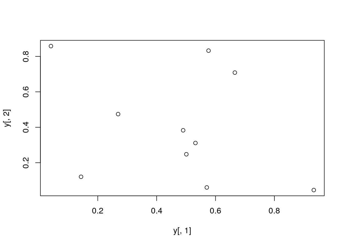
Plot data
plot(y[,1], y[,2])
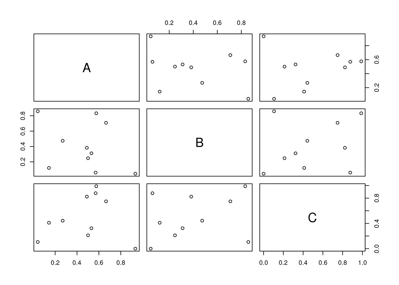
All pairs
pairs(y)
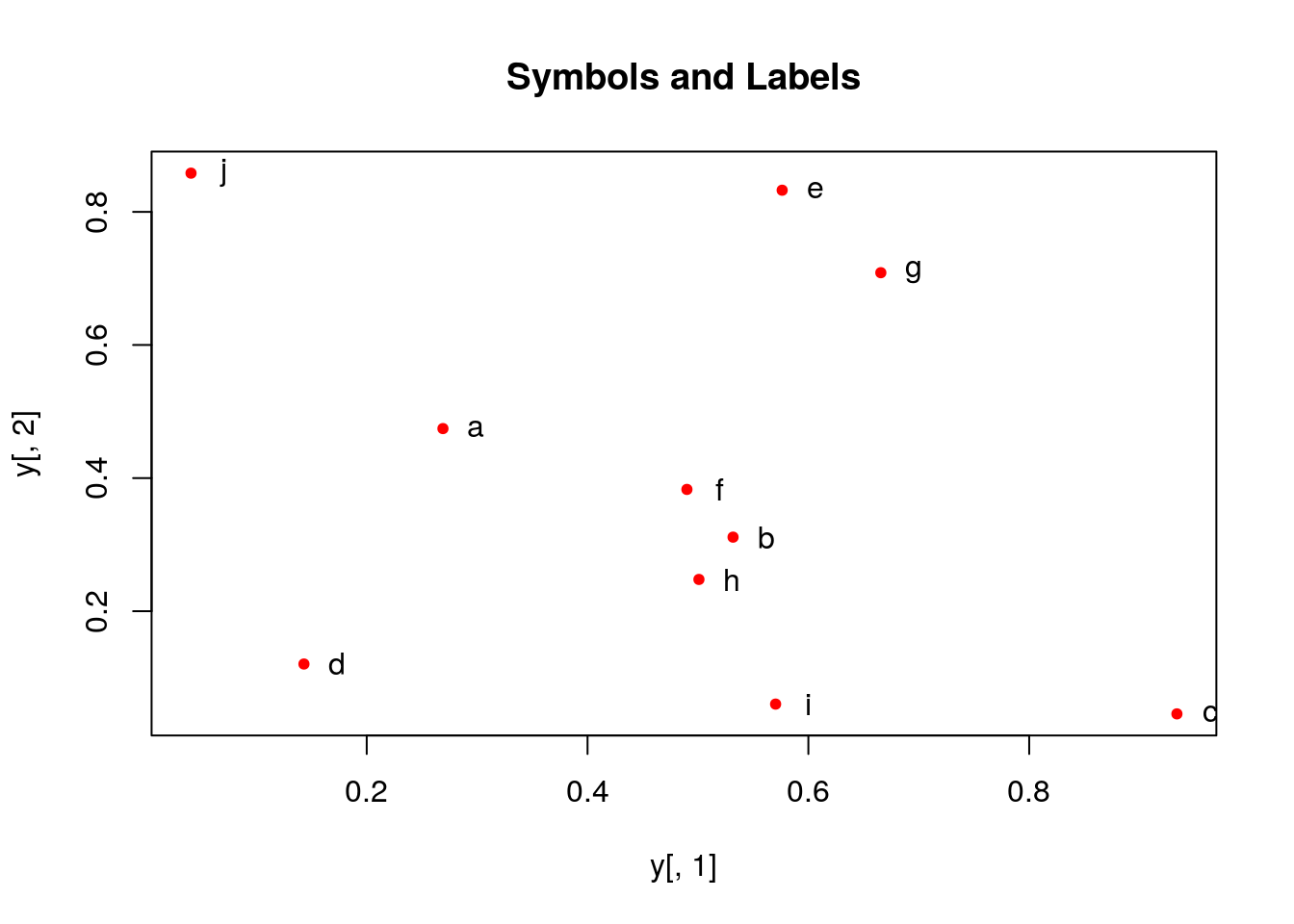
With labels
plot(y[,1], y[,2], pch=20, col="red", main="Symbols and Labels")
text(y[,1]+0.03, y[,2], rownames(y))
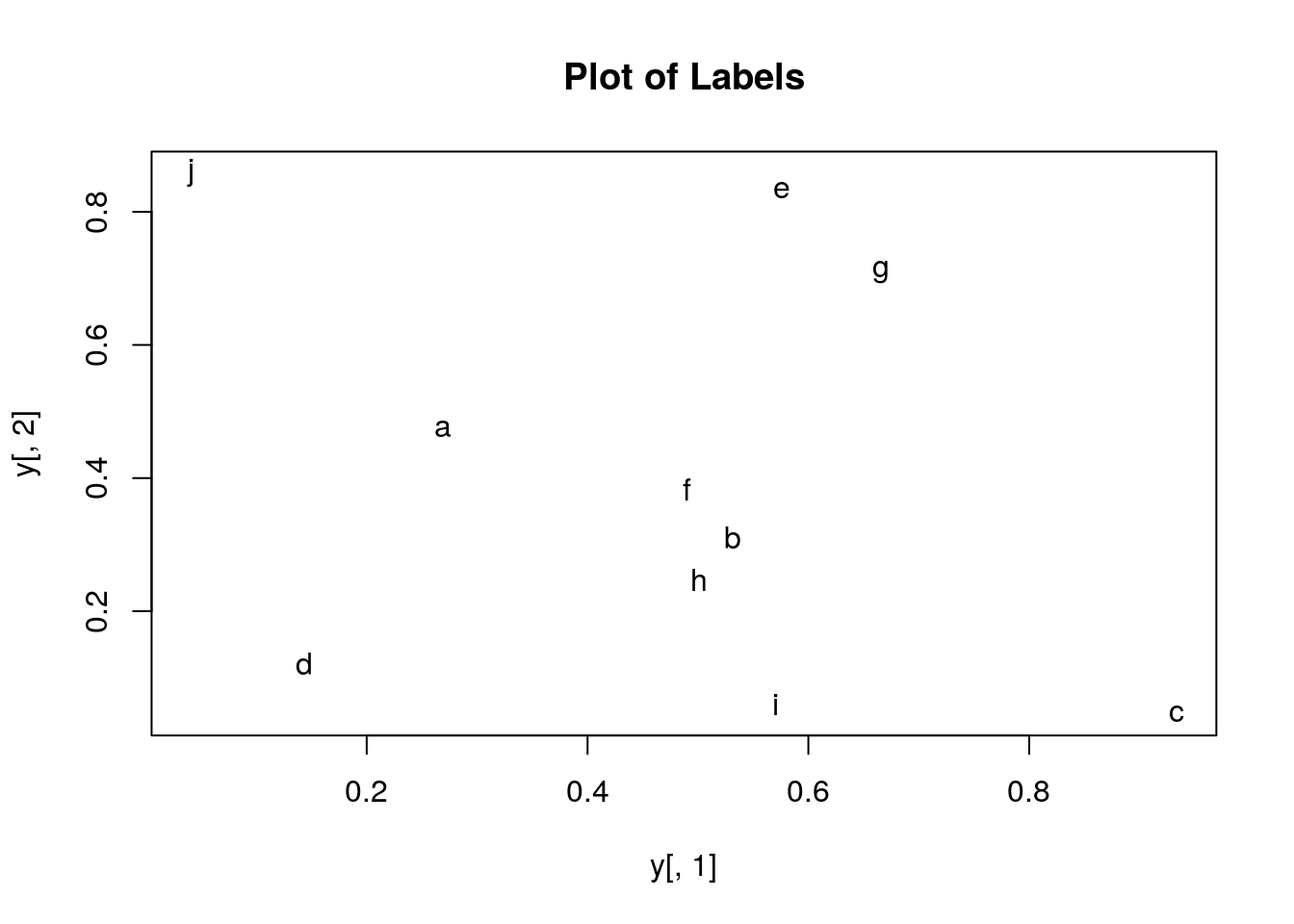
More examples
Print instead of symbols the row names
plot(y[,1], y[,2], type="n", main="Plot of Labels")
text(y[,1], y[,2], rownames(y))
Usage of important plotting parameters
grid(5, 5, lwd = 2)
op <- par(mar=c(8,8,8,8), bg="lightblue")
plot(y[,1], y[,2], type="p", col="red", cex.lab=1.2, cex.axis=1.2,
     cex.main=1.2, cex.sub=1, lwd=4, pch=20, xlab="x label",
     ylab="y label", main="My Main", sub="My Sub")
par(op)
Important arguments
mar: specifies the margin sizes around the plotting area in order:c(bottom, left, top, right)col: color of symbolspch: type of symbols, samples:example(points)lwd: size of symbolscex.*: control font sizes- For details see
?par
Add regression line
plot(y[,1], y[,2])
myline <- lm(y[,2]~y[,1]); abline(myline, lwd=2)
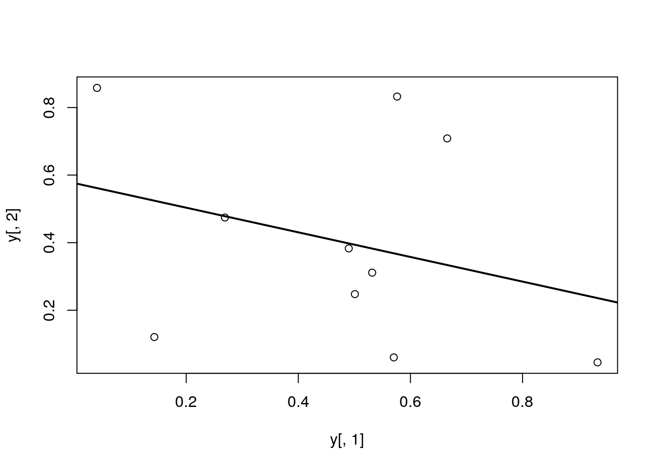
summary(myline)
##
## Call:
## lm(formula = y[, 2] ~ y[, 1])
##
## Residuals:
##      Min       1Q   Median       3Q      Max
## -0.40357 -0.17912 -0.04299  0.22147  0.46623
##
## Coefficients:
##             Estimate Std. Error t value Pr(>|t|)
## (Intercept)   0.5764     0.2110   2.732   0.0258 *
## y[, 1]       -0.3647     0.3959  -0.921   0.3839
## ---
## Signif. codes:  0 '***' 0.001 '**' 0.01 '*' 0.05 '.' 0.1 ' ' 1
##
## Residual standard error: 0.3095 on 8 degrees of freedom
## Multiple R-squared:  0.09589,	Adjusted R-squared:  -0.01712
## F-statistic: 0.8485 on 1 and 8 DF,  p-value: 0.3839
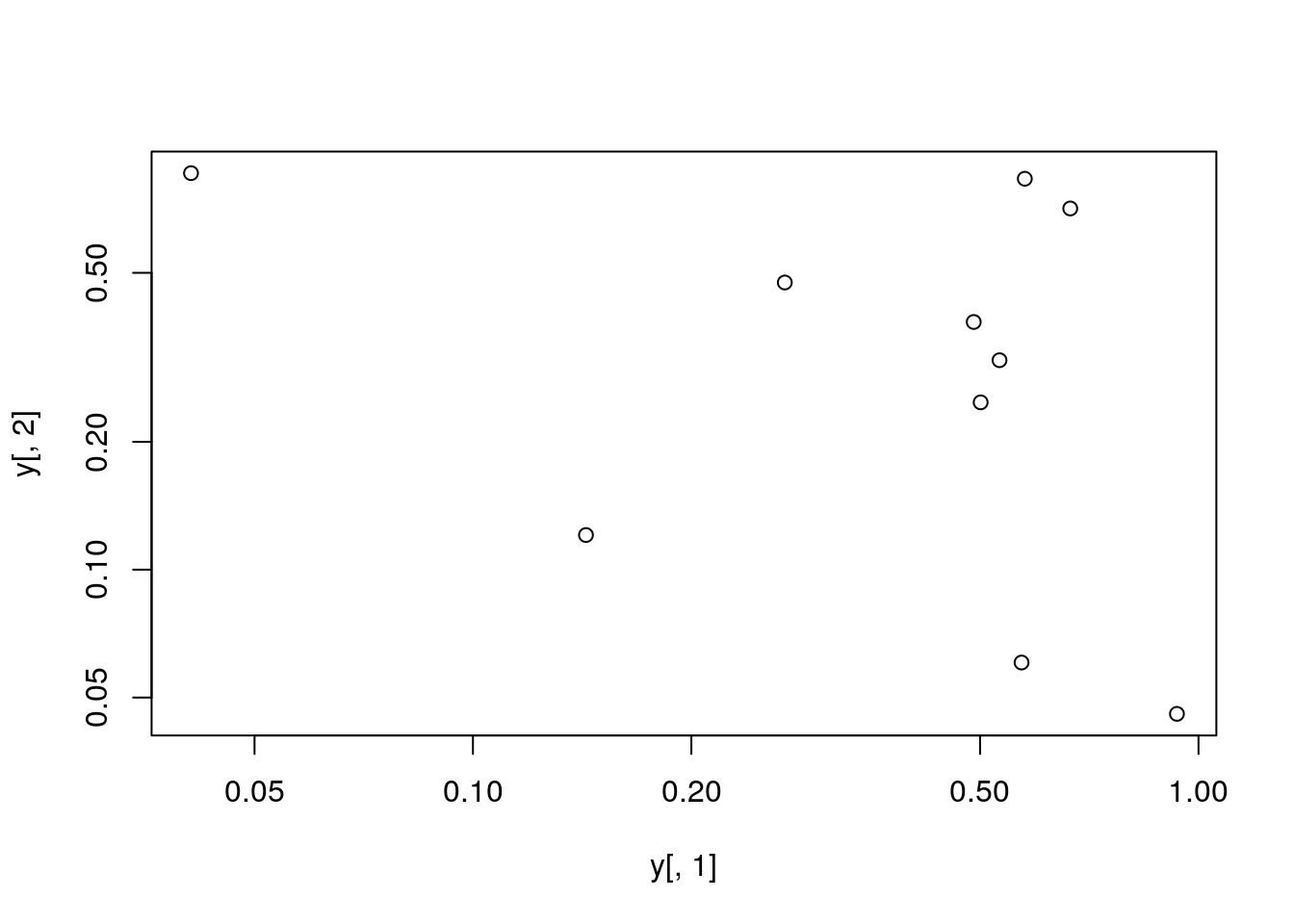
Log scale
Same plot as above, but on log scale
plot(y[,1], y[,2], log="xy")
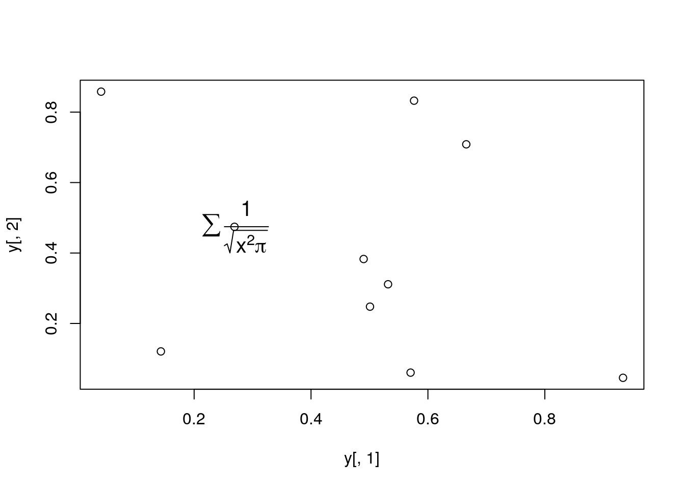
Add a mathematical expression
plot(y[,1], y[,2]); text(y[1,1], y[1,2], expression(sum(frac(1,sqrt(x^2*pi)))), cex=1.3)
Homework 3B
Homework 3B: Scatter Plots
Line Plots
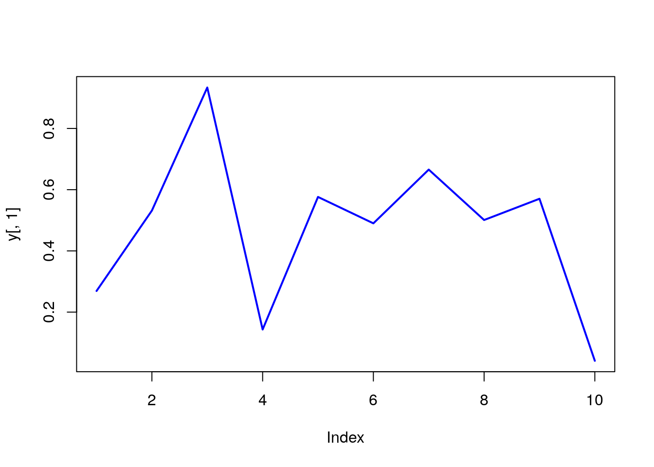
Single data set
plot(y[,1], type="l", lwd=2, col="blue")
Many Data Sets
Plots line graph for all columns in data frame y. The split.screen function is used in this example in a for loop to overlay several line graphs in the same plot.
split.screen(c(1,1))
## [1] 1
plot(y[,1], ylim=c(0,1), xlab="Measurement", ylab="Intensity", type="l", lwd=2, col=1)
for(i in 2:length(y[1,])) {
	screen(1, new=FALSE)
	plot(y[,i], ylim=c(0,1), type="l", lwd=2, col=i, xaxt="n", yaxt="n", ylab="", xlab="", main="", bty="n")
}
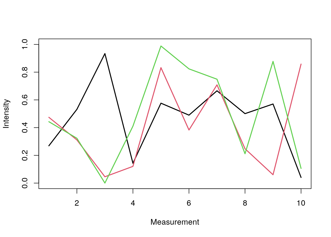
close.screen(all=TRUE)
Bar Plots
Basics
barplot(y[1:4,], ylim=c(0, max(y[1:4,])+0.3), beside=TRUE, legend=letters[1:4])
text(labels=round(as.vector(as.matrix(y[1:4,])),2), x=seq(1.5, 13, by=1) + sort(rep(c(0,1,2), 4)), y=as.vector(as.matrix(y[1:4,]))+0.04)
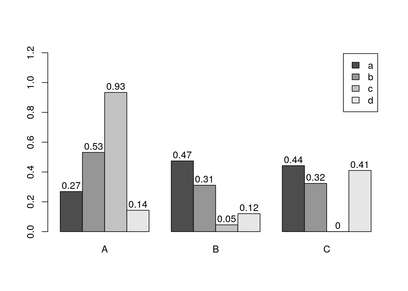
The barplot function has a convenient default behavior when the input data are provided as matrix containing row and column names. The column names are used in the barplot as group labels (here A to C) and the row names as labels for each measurement within a group (here: a to d). When working with a data.frame or tibble, use as.matrix to coerce the input to a matrix; and to populate or change the rownames or colnames slots, use rownames(y) <- ... or colnames(y) <- ..., respectively.
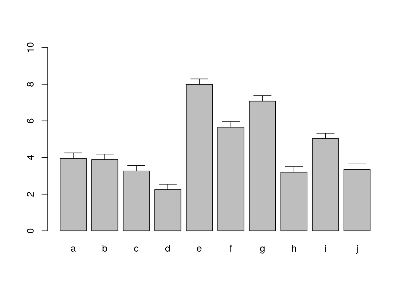
Error Bars
bar <- barplot(m <- rowMeans(y) * 10, ylim=c(0, 10))
stdev <- sd(t(y))
arrows(bar, m, bar, m + stdev, length=0.15, angle = 90)
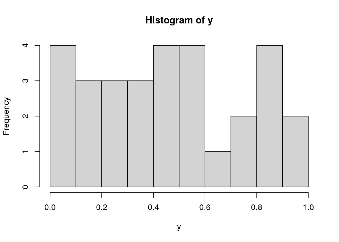
Histograms
hist(y, freq=TRUE, breaks=10)
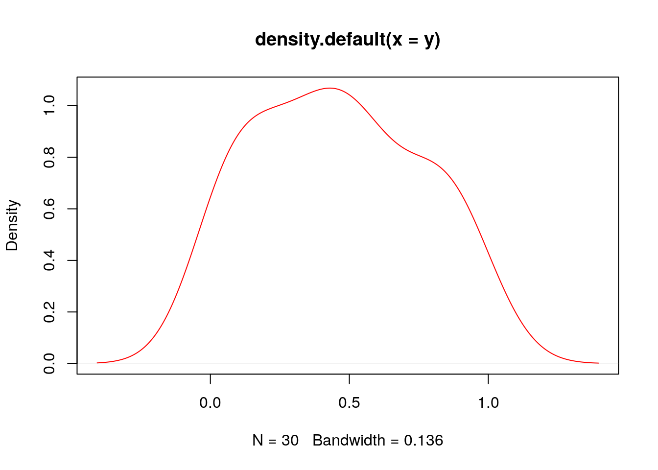
Density Plots
plot(density(y), col="red")
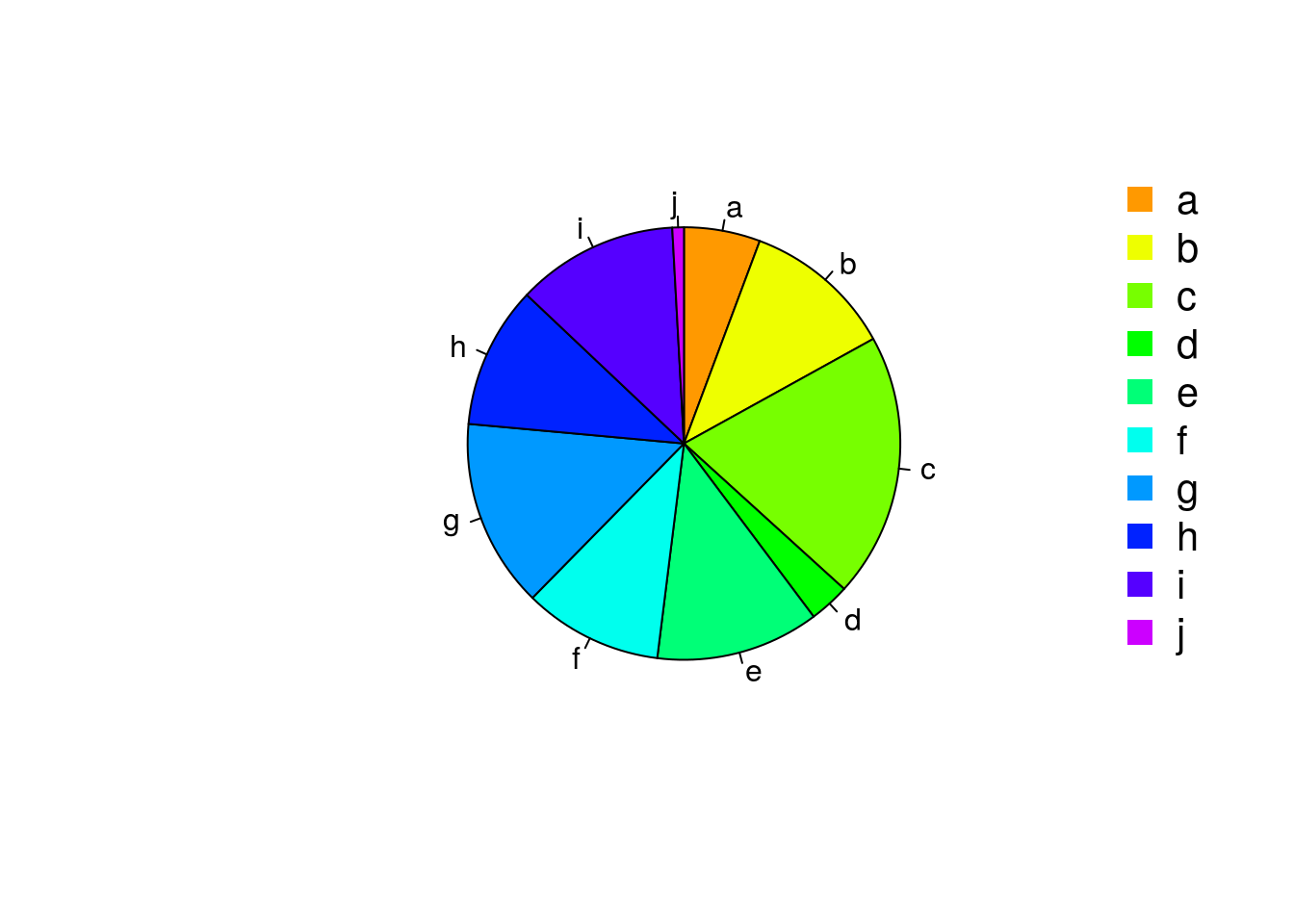
Pie Charts
pie(y[,1], col=rainbow(length(y[,1]), start=0.1, end=0.8), clockwise=TRUE)
legend("topright", legend=row.names(y), cex=1.3, bty="n", pch=15, pt.cex=1.8,
col=rainbow(length(y[,1]), start=0.1, end=0.8), ncol=1)
Color Selection Utilities
Default color palette and how to change it
palette()
## [1] "black" "#DF536B" "#61D04F" "#2297E6" "#28E2E5" "#CD0BBC" "#F5C710" "gray62"
palette(rainbow(5, start=0.1, end=0.2))
palette()
## [1] "#FF9900" "#FFBF00" "#FFE600" "#F2FF00" "#CCFF00"
palette("default")
The gray function allows to select any type of gray shades by providing values from 0 to 1
gray(seq(0.1, 1, by= 0.2))
## [1] "#1A1A1A" "#4D4D4D" "#808080" "#B3B3B3" "#E6E6E6"
Color gradients with colorpanel function from gplots library`
library(gplots)
colorpanel(5, "darkblue", "yellow", "white")
## [1] "#00008B" "#808046" "#FFFF00" "#FFFF80" "#FFFFFF"
Much more on colors in R see Earl Glynn’s color chart here
Saving Graphics to File
After the pdf() command all graphs are redirected to file test.pdf. Works for all common formats similarly: jpeg, png, ps, tiff, …
pdf("test.pdf")
plot(1:10, 1:10)
dev.off()
Generates Scalable Vector Graphics (SVG) files that can be edited in vector graphics programs, such as InkScape.
library("RSvgDevice")
devSVG("test.svg")
plot(1:10, 1:10)
dev.off()
Homework 3C
Homework 3C: Bar Plots
Analysis Routine
Overview
The following exercise introduces a variety of useful data analysis utilities in R.
Analysis Routine: Data Import
-
Step 1: To get started with this exercise, direct your R session to a dedicated workshop directory and download into this directory the following sample tables. Then import the files into Excel and save them as tab delimited text files.
Import the tables into R
Import molecular weight table
my_mw <- read.delim(file="MolecularWeight_tair7.xls", header=TRUE, sep="\t")
my_mw[1:2,]
Import subcelluar targeting table
my_target <- read.delim(file="TargetP_analysis_tair7.xls", header=TRUE, sep="\t")
my_target[1:2,]
Online import of molecular weight table
my_mw <- read.delim(file="http://faculty.ucr.edu/~tgirke/Documents/R_BioCond/Samples/MolecularWeight_tair7.xls", header=TRUE, sep="\t")
my_mw[1:2,]
##   Sequence.id Molecular.Weight.Da. Residues
## 1 AT1G08520.1                83285      760
## 2 AT1G08530.1                27015      257
Online import of subcelluar targeting table
my_target <- read.delim(file="http://faculty.ucr.edu/~tgirke/Documents/R_BioCond/Samples/TargetP_analysis_tair7.xls", header=TRUE, sep="\t")
my_target[1:2,]
##      GeneName Loc   cTP   mTP    SP other
## 1 AT1G08520.1   C 0.822 0.137 0.029 0.039
## 2 AT1G08530.1   C 0.817 0.058 0.010 0.100
Merging Data Frames
- Step 2: Assign uniform gene ID column titles
colnames(my_target)[1] <- "ID"
colnames(my_mw)[1] <- "ID"
- Step 3: Merge the two tables based on common ID field
my_mw_target <- merge(my_mw, my_target, by.x="ID", by.y="ID", all.x=TRUE)
- Step 4: Shorten one table before the merge and then remove the non-matching rows (NAs) in the merged file
my_mw_target2a <- merge(my_mw, my_target[1:40,], by.x="ID", by.y="ID", all.x=TRUE)  # To remove non-matching rows, use the argument setting 'all=FALSE'.
my_mw_target2 <- na.omit(my_mw_target2a) # Removes rows containing "NAs" (non-matching rows).
- Homework 3D: How can the merge function in the previous step be executed so that only the common rows among the two data frames are returned? Prove that both methods - the two step version with
na.omitand your method - return identical results. - Homework 3E: Replace all
NAsin the data framemy_mw_target2awith zeros.
Filtering Data
- Step 5: Retrieve all records with a value of greater than 100,000 in ‘MW’ column and ‘C’ value in ‘Loc’ column (targeted to chloroplast).
query <- my_mw_target[my_mw_target[, 2] > 100000 & my_mw_target[, 4] == "C", ]
query[1:4, ]
##              ID Molecular.Weight.Da. Residues Loc   cTP   mTP    SP other
## 219 AT1G02730.1               132588     1181   C 0.972 0.038 0.008 0.045
## 243 AT1G02890.1               136825     1252   C 0.748 0.529 0.011 0.013
## 281 AT1G03160.1               100732      912   C 0.871 0.235 0.011 0.007
## 547 AT1G05380.1               126360     1138   C 0.740 0.099 0.016 0.358
dim(query)
## [1] 170 8
- Homework 3F: How many protein entries in the
my_mw_targetdata frame have a MW of greater then 4,000 and less then 5,000. Subset the data frame accordingly and sort it by MW to check that your result is correct.
String Substitutions
- Step 6: Use a regular expression in a substitute function to generate a separate ID column that lacks the gene model extensions.
my_mw_target3 <- data.frame(loci=gsub("\\..*", "", as.character(my_mw_target[,1]), perl = TRUE), my_mw_target)
my_mw_target3[1:3,1:8]
##        loci          ID Molecular.Weight.Da. Residues Loc  cTP   mTP    SP
## 1 AT1G01010 AT1G01010.1                49426      429   _ 0.10 0.090 0.075
## 2 AT1G01020 AT1G01020.1                28092      245   * 0.01 0.636 0.158
## 3 AT1G01020 AT1G01020.2                21711      191   * 0.01 0.636 0.158
- Homework 3G: Retrieve those rows in
my_mw_target3where the second column contains the following identifiers:c("AT5G52930.1", "AT4G18950.1", "AT1G15385.1", "AT4G36500.1", "AT1G67530.1"). Use the%in%function for this query. As an alternative approach, assign the second column to the row index of the data frame and then perform the same query again using the row index. Explain the difference of the two methods.
Calculations on Data Frames
- Step 7: Count the number of duplicates in the loci column with the
tablefunction and append the result to the data frame with thecbindfunction.
mycounts <- table(my_mw_target3[,1])[my_mw_target3[,1]]
my_mw_target4 <- cbind(my_mw_target3, Freq=mycounts[as.character(my_mw_target3[,1])])
- Step 8: Perform a vectorized devision of columns 3 and 4 (average AA weight per protein)
data.frame(my_mw_target4, avg_AA_WT=(my_mw_target4[,3] / my_mw_target4[,4]))[1:2,]
##        loci          ID Molecular.Weight.Da. Residues Loc  cTP   mTP    SP other Freq.Var1
## 1 AT1G01010 AT1G01010.1                49426      429   _ 0.10 0.090 0.075 0.925 AT1G01010
## 2 AT1G01020 AT1G01020.1                28092      245   * 0.01 0.636 0.158 0.448 AT1G01020
##   Freq.Freq avg_AA_WT
## 1         1  115.2121
## 2         2  114.6612
- Step 9: Calculate for each row the mean and standard deviation across several columns
mymean <- apply(my_mw_target4[,6:9], 1, mean)
mystdev <- apply(my_mw_target4[,6:9], 1, sd, na.rm=TRUE)
data.frame(my_mw_target4, mean=mymean, stdev=mystdev)[1:2,5:12]
##   Loc  cTP   mTP    SP other Freq.Var1 Freq.Freq   mean
## 1   _ 0.10 0.090 0.075 0.925 AT1G01010         1 0.2975
## 2   * 0.01 0.636 0.158 0.448 AT1G01020         2 0.3130
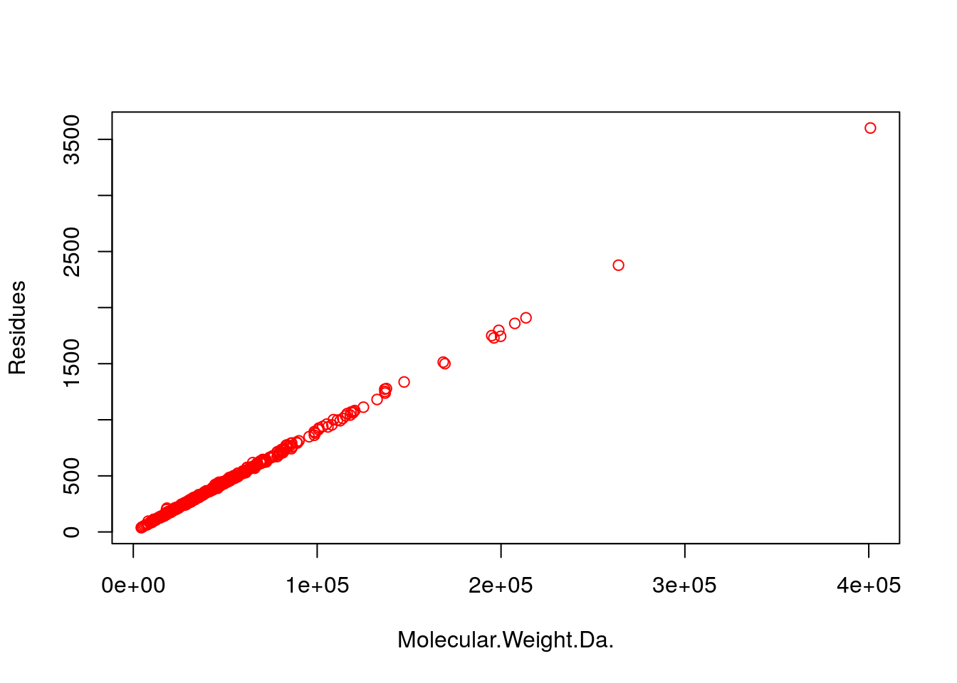
Plotting Example
- Step 10: Generate scatter plot for the ‘MW’ and ‘Residues’ columns.
plot(my_mw_target4[1:500,3:4], col="red")
Export Results and Run Entire Exercise as Script
- Step 11: Write the data frame
my_mw_target4into a tab-delimited text file and inspect it in Excel.
write.table(my_mw_target4, file="my_file.xls", quote=FALSE, sep="\t", col.names = NA)
- Homework 3H: Write all commands from this exercise into an R script named
exerciseRbasics.R, or download it from here. For demonstration the downloadable script version contains code for generating some additional plots that are not part of this exercise. Then execute the script with thesourcefunction like this:source("exerciseRbasics.R"). This will run all commands of this exercise and generate the corresponding output files in the current working directory. For homework 3H it is not necessary to submit the result files generated by theexerciseRbasics.Rscript. Stating how the script was executed (e.g.sourceorRscriptcommand) will be sufficient.
source("exerciseRbasics.R")
Or run it from the command-line (not from R!) with Rscript like this:
Rscript exerciseRbasics.R
Miscellaneous Topics
Upgrading to New R/Bioc Versions
When upgrading to a new R version, it is important to understand that a reinstall of all R packages is necessary because CRAN/Bioc packages are developed and tested for specific R versions. This means when upgrading R, then the corresponding packages need to be upgraded to the versions that match the new R version. The following steps will work in many situations.
-
Export a list of all packages installed in a current version of R to a file (below named
my_R_pkgs.txt) by running the following commands from within R (or useRscript -efrom command-line)my_R_pkgs <- rownames(installed.packages()) writeLines(my_R_pkgs, "my_R_pkgs.txt") -
Install new version of R, and then from within the new R version all packages one had installed before. The first install command below installs first a series of packages that are useful to have in general no matter what. Custom packages are then installed in the next lines. Note, this can only install packages from CRAN and Bioconductor. Packages from custom sources, including private GitHub accounts, need to be installed separately. Usually, one can identify them by the report generated at the end of the below install routine telling which packages are not available on CRAN or Bioconductor.
install.packages(c("devtools", "tidyverse", "BiocManager"))
BiocManager::install(version = "3.19") # look up current Bioc version here: https://bit.ly/3NADnll
my_R_pkgs <- readLines("my_R_pkgs.txt")
BiocManager::install(my_R_pkgs)
Session Info
sessionInfo()
## R version 4.1.3 (2022-03-10)
## Platform: x86_64-pc-linux-gnu (64-bit)
## Running under: Debian GNU/Linux 10 (buster)
##
## Matrix products: default
## BLAS:   /usr/lib/x86_64-linux-gnu/blas/libblas.so.3.8.0
## LAPACK: /usr/lib/x86_64-linux-gnu/lapack/liblapack.so.3.8.0
##
## locale:
##  [1] LC_CTYPE=en_US.UTF-8       LC_NUMERIC=C               LC_TIME=en_US.UTF-8
##  [4] LC_COLLATE=en_US.UTF-8     LC_MONETARY=en_US.UTF-8    LC_MESSAGES=en_US.UTF-8
##  [7] LC_PAPER=en_US.UTF-8       LC_NAME=C                  LC_ADDRESS=C
## [10] LC_TELEPHONE=C             LC_MEASUREMENT=en_US.UTF-8 LC_IDENTIFICATION=C
##
## attached base packages:
## [1] stats     graphics  grDevices utils     datasets  methods   base
##
## other attached packages:
##  [1] gplots_3.1.1     forcats_0.5.1    stringr_1.4.0    dplyr_1.0.7      purrr_0.3.4
##  [6] readr_2.1.1      tidyr_1.1.4      tibble_3.1.6     tidyverse_1.3.1  ggplot2_3.3.5
## [11] limma_3.50.0     BiocStyle_2.22.0
##
## loaded via a namespace (and not attached):
##  [1] Rcpp_1.0.8.3        lubridate_1.8.0     gtools_3.9.2        assertthat_0.2.1
##  [5] digest_0.6.29       utf8_1.2.2          R6_2.5.1            cellranger_1.1.0
##  [9] backports_1.4.0     reprex_2.0.1        evaluate_0.15       highr_0.9
## [13] httr_1.4.2          blogdown_1.8.2      pillar_1.6.4        rlang_1.0.2
## [17] readxl_1.3.1        rstudioapi_0.13     jquerylib_0.1.4     rmarkdown_2.13
## [21] munsell_0.5.0       broom_0.7.10        compiler_4.1.3      modelr_0.1.8
## [25] xfun_0.30           pkgconfig_2.0.3     htmltools_0.5.2     tidyselect_1.1.1
## [29] bookdown_0.25       codetools_0.2-18    fansi_0.5.0         crayon_1.4.2
## [33] tzdb_0.2.0          dbplyr_2.1.1        withr_2.4.3         bitops_1.0-7
## [37] grid_4.1.3          jsonlite_1.8.0      gtable_0.3.0        lifecycle_1.0.1
## [41] DBI_1.1.1           magrittr_2.0.2      scales_1.1.1        KernSmooth_2.23-20
## [45] cli_3.1.0           stringi_1.7.6       fs_1.5.2            xml2_1.3.3
## [49] bslib_0.3.1         ellipsis_0.3.2      generics_0.1.1      vctrs_0.3.8
## [53] tools_4.1.3         glue_1.6.2          hms_1.1.1           fastmap_1.1.0
## [57] yaml_2.3.5          colorspace_2.0-2    BiocManager_1.30.16 caTools_1.18.2
## [61] rvest_1.0.2         knitr_1.37          haven_2.4.3         sass_0.4.0