Tidyverse and Some SQLite
23 minute read
Overview
Modern object classes and methods for handling data.frame like structures
are provided by the dplyr (tidyr) and data.table packages. A related example is Bioconductor’s
DataTable object class (“Learn the tidyverse,” n.d.). This tutorial provide a short introduction to the usage and
functionalities of the dplyr and related packages.
Related documentation
More detailed tutorials on this topic can be found here:
- dplyr: A Grammar of Data Manipulation
- Introduction to
dplyr - Tutorial on
dplyr - Cheatsheet for Joins from Jenny Bryan
- Tibbles
- Intro to
data.tablepackage - Big data with
dplyranddata.table - Fast lookups with
dplyranddata.table
Installation
The dplyr (tidyr) environment has evolved into an ecosystem of packages. To simplify
package management, one can install and load the entire collection via the
tidyverse package. For more details on tidyverse see
here.
install.packages("tidyverse")
Construct a tibble (tibble)
library(tidyverse)
as_tibble(iris) # coerce data.frame to tibble tbl
## # A tibble: 150 × 5
##    Sepal.Length Sepal.Width Petal.Length Petal.Width Species
##           <dbl>       <dbl>        <dbl>       <dbl> <fct>
##  1          5.1         3.5          1.4         0.2 setosa
##  2          4.9         3            1.4         0.2 setosa
##  3          4.7         3.2          1.3         0.2 setosa
##  4          4.6         3.1          1.5         0.2 setosa
##  5          5           3.6          1.4         0.2 setosa
##  6          5.4         3.9          1.7         0.4 setosa
##  7          4.6         3.4          1.4         0.3 setosa
##  8          5           3.4          1.5         0.2 setosa
##  9          4.4         2.9          1.4         0.2 setosa
## 10          4.9         3.1          1.5         0.1 setosa
## # … with 140 more rows
Reading and writing tabular files
While the base R read/write utilities can be used for data.frames, best time
performance with the least amount of typing is achieved with the export/import
functions from the readr package. For very large files the fread function from
the data.table package achieves the best time performance.
Import with readr
Import functions provided by readr include:
read_csv(): comma separated (CSV) filesread_tsv(): tab separated filesread_delim(): general delimited filesread_fwf(): fixed width filesread_table(): tabular files where colums are separated by white-space.read_log(): web log files
Create a sample tab delimited file for import
write_tsv(iris, "iris.txt") # Creates sample file
Import with read_tsv
iris_df <- read_tsv("iris.txt") # Import with read_tbv from readr package
iris_df
## # A tibble: 150 × 5
##    Sepal.Length Sepal.Width Petal.Length Petal.Width Species
##           <dbl>       <dbl>        <dbl>       <dbl> <chr>
##  1          5.1         3.5          1.4         0.2 setosa
##  2          4.9         3            1.4         0.2 setosa
##  3          4.7         3.2          1.3         0.2 setosa
##  4          4.6         3.1          1.5         0.2 setosa
##  5          5           3.6          1.4         0.2 setosa
##  6          5.4         3.9          1.7         0.4 setosa
##  7          4.6         3.4          1.4         0.3 setosa
##  8          5           3.4          1.5         0.2 setosa
##  9          4.4         2.9          1.4         0.2 setosa
## 10          4.9         3.1          1.5         0.1 setosa
## # … with 140 more rows
To import Google Sheets directly into R, see here.
Fast table import with fread
The fread function from the data.table package provides the best time performance for reading large
tabular files into R.
library(data.table)
iris_df <- as_tibble(fread("iris.txt")) # Import with fread and conversion to tibble
iris_df
## # A tibble: 150 × 5
##    Sepal.Length Sepal.Width Petal.Length Petal.Width Species
##           <dbl>       <dbl>        <dbl>       <dbl> <chr>
##  1          5.1         3.5          1.4         0.2 setosa
##  2          4.9         3            1.4         0.2 setosa
##  3          4.7         3.2          1.3         0.2 setosa
##  4          4.6         3.1          1.5         0.2 setosa
##  5          5           3.6          1.4         0.2 setosa
##  6          5.4         3.9          1.7         0.4 setosa
##  7          4.6         3.4          1.4         0.3 setosa
##  8          5           3.4          1.5         0.2 setosa
##  9          4.4         2.9          1.4         0.2 setosa
## 10          4.9         3.1          1.5         0.1 setosa
## # … with 140 more rows
Note: to ignore lines starting with comment signs, one can pass on to fread a shell
command for preprocessing the file. The following example illustrates this option.
fread("grep -v '^#' iris.txt")
Export with readr
Export function provided by readr inlcude
write_delim(): general delimited fileswrite_csv(): comma separated (CSV) fileswrite_excel_csv(): excel style CSV fileswrite_tsv(): tab separated files
For instance, the write_tsv function writes a data.frame or tibble to a tab delimited file with much nicer
default settings than the base R write.table function.
write_tsv(iris_df, "iris.txt")
Column and row binds
The equivalents to base R’s rbind and cbind are bind_rows and bind_cols, respectively.
bind_cols(iris_df, iris_df)
## # A tibble: 150 × 10
##    Sepal.Length...1 Sepal.Width...2 Petal.Length...3 Petal.Width...4 Species...5 Sepal.Length...6
##               <dbl>           <dbl>            <dbl>           <dbl> <chr>                  <dbl>
##  1              5.1             3.5              1.4             0.2 setosa                   5.1
##  2              4.9             3                1.4             0.2 setosa                   4.9
##  3              4.7             3.2              1.3             0.2 setosa                   4.7
##  4              4.6             3.1              1.5             0.2 setosa                   4.6
##  5              5               3.6              1.4             0.2 setosa                   5
##  6              5.4             3.9              1.7             0.4 setosa                   5.4
##  7              4.6             3.4              1.4             0.3 setosa                   4.6
##  8              5               3.4              1.5             0.2 setosa                   5
##  9              4.4             2.9              1.4             0.2 setosa                   4.4
## 10              4.9             3.1              1.5             0.1 setosa                   4.9
## # … with 140 more rows, and 4 more variables: Sepal.Width...7 <dbl>, Petal.Length...8 <dbl>,
## #   Petal.Width...9 <dbl>, Species...10 <chr>
bind_rows(iris_df, iris_df)
## # A tibble: 300 × 5
##    Sepal.Length Sepal.Width Petal.Length Petal.Width Species
##           <dbl>       <dbl>        <dbl>       <dbl> <chr>
##  1          5.1         3.5          1.4         0.2 setosa
##  2          4.9         3            1.4         0.2 setosa
##  3          4.7         3.2          1.3         0.2 setosa
##  4          4.6         3.1          1.5         0.2 setosa
##  5          5           3.6          1.4         0.2 setosa
##  6          5.4         3.9          1.7         0.4 setosa
##  7          4.6         3.4          1.4         0.3 setosa
##  8          5           3.4          1.5         0.2 setosa
##  9          4.4         2.9          1.4         0.2 setosa
## 10          4.9         3.1          1.5         0.1 setosa
## # … with 290 more rows
Extract column as vector
The subsetting operators [[ and $can be used to extract from a tibble single columns as vector.
iris_df[[5]][1:12]
##  [1] "setosa" "setosa" "setosa" "setosa" "setosa" "setosa" "setosa" "setosa" "setosa" "setosa"
## [11] "setosa" "setosa"
iris_df$Species[1:12]
##  [1] "setosa" "setosa" "setosa" "setosa" "setosa" "setosa" "setosa" "setosa" "setosa" "setosa"
## [11] "setosa" "setosa"
Important dplyr functions
filter()andslice()arrange()select()andrename()distinct()mutate()andtransmute()summarise()sample_n()andsample_frac()
Slice and filter functions
Filter function
filter(iris_df, Sepal.Length > 7.5, Species=="virginica")
## # A tibble: 6 × 5
##   Sepal.Length Sepal.Width Petal.Length Petal.Width Species
##          <dbl>       <dbl>        <dbl>       <dbl> <chr>
## 1          7.6         3            6.6         2.1 virginica
## 2          7.7         3.8          6.7         2.2 virginica
## 3          7.7         2.6          6.9         2.3 virginica
## 4          7.7         2.8          6.7         2   virginica
## 5          7.9         3.8          6.4         2   virginica
## 6          7.7         3            6.1         2.3 virginica
Base R code equivalent
iris_df[iris_df[, "Sepal.Length"] > 7.5 & iris_df[, "Species"]=="virginica", ]
## # A tibble: 6 × 5
##   Sepal.Length Sepal.Width Petal.Length Petal.Width Species
##          <dbl>       <dbl>        <dbl>       <dbl> <chr>
## 1          7.6         3            6.6         2.1 virginica
## 2          7.7         3.8          6.7         2.2 virginica
## 3          7.7         2.6          6.9         2.3 virginica
## 4          7.7         2.8          6.7         2   virginica
## 5          7.9         3.8          6.4         2   virginica
## 6          7.7         3            6.1         2.3 virginica
Including boolean operators
filter(iris_df, Sepal.Length > 7.5 | Sepal.Length < 5.5, Species=="virginica")
## # A tibble: 7 × 5
##   Sepal.Length Sepal.Width Petal.Length Petal.Width Species
##          <dbl>       <dbl>        <dbl>       <dbl> <chr>
## 1          7.6         3            6.6         2.1 virginica
## 2          4.9         2.5          4.5         1.7 virginica
## 3          7.7         3.8          6.7         2.2 virginica
## 4          7.7         2.6          6.9         2.3 virginica
## 5          7.7         2.8          6.7         2   virginica
## 6          7.9         3.8          6.4         2   virginica
## 7          7.7         3            6.1         2.3 virginica
Subset rows by position
dplyr approach
slice(iris_df, 1:2)
## # A tibble: 2 × 5
##   Sepal.Length Sepal.Width Petal.Length Petal.Width Species
##          <dbl>       <dbl>        <dbl>       <dbl> <chr>
## 1          5.1         3.5          1.4         0.2 setosa
## 2          4.9         3            1.4         0.2 setosa
Base R code equivalent
iris_df[1:2,]
## # A tibble: 2 × 5
##   Sepal.Length Sepal.Width Petal.Length Petal.Width Species
##          <dbl>       <dbl>        <dbl>       <dbl> <chr>
## 1          5.1         3.5          1.4         0.2 setosa
## 2          4.9         3            1.4         0.2 setosa
Subset rows by names
Since tibbles do not contain row names, row wise subsetting via the [,] operator cannot be used.
However, the corresponding behavior can be achieved by passing to select a row position index
obtained by basic R intersect utilities such as match.
Create a suitable test tibble
df1 <- bind_cols(tibble(ids1=paste0("g", 1:10)), as_tibble(matrix(1:40, 10, 4, dimnames=list(1:10, paste0("CA", 1:4)))))
df1
## # A tibble: 10 × 5
##    ids1    CA1   CA2   CA3   CA4
##    <chr> <int> <int> <int> <int>
##  1 g1        1    11    21    31
##  2 g2        2    12    22    32
##  3 g3        3    13    23    33
##  4 g4        4    14    24    34
##  5 g5        5    15    25    35
##  6 g6        6    16    26    36
##  7 g7        7    17    27    37
##  8 g8        8    18    28    38
##  9 g9        9    19    29    39
## 10 g10      10    20    30    40
dplyr approach
slice(df1, match(c("g10", "g4", "g4"), ids1))
## # A tibble: 3 × 5
##   ids1    CA1   CA2   CA3   CA4
##   <chr> <int> <int> <int> <int>
## 1 g10      10    20    30    40
## 2 g4        4    14    24    34
## 3 g4        4    14    24    34
Base R equivalent
df1_old <- as.data.frame(df1)
rownames(df1_old) <- df1_old[,1]
df1_old[c("g10", "g4", "g4"),]
##      ids1 CA1 CA2 CA3 CA4
## g10   g10  10  20  30  40
## g4     g4   4  14  24  34
## g4.1   g4   4  14  24  34
Sorting with arrange
Row-wise ordering based on specific columns
dplyr approach
arrange(iris_df, Species, Sepal.Length, Sepal.Width)
## # A tibble: 150 × 5
##    Sepal.Length Sepal.Width Petal.Length Petal.Width Species
##           <dbl>       <dbl>        <dbl>       <dbl> <chr>
##  1          4.3         3            1.1         0.1 setosa
##  2          4.4         2.9          1.4         0.2 setosa
##  3          4.4         3            1.3         0.2 setosa
##  4          4.4         3.2          1.3         0.2 setosa
##  5          4.5         2.3          1.3         0.3 setosa
##  6          4.6         3.1          1.5         0.2 setosa
##  7          4.6         3.2          1.4         0.2 setosa
##  8          4.6         3.4          1.4         0.3 setosa
##  9          4.6         3.6          1           0.2 setosa
## 10          4.7         3.2          1.3         0.2 setosa
## # … with 140 more rows
For ordering descendingly use desc() function
arrange(iris_df, desc(Species), Sepal.Length, Sepal.Width)
## # A tibble: 150 × 5
##    Sepal.Length Sepal.Width Petal.Length Petal.Width Species
##           <dbl>       <dbl>        <dbl>       <dbl> <chr>
##  1          4.9         2.5          4.5         1.7 virginica
##  2          5.6         2.8          4.9         2   virginica
##  3          5.7         2.5          5           2   virginica
##  4          5.8         2.7          5.1         1.9 virginica
##  5          5.8         2.7          5.1         1.9 virginica
##  6          5.8         2.8          5.1         2.4 virginica
##  7          5.9         3            5.1         1.8 virginica
##  8          6           2.2          5           1.5 virginica
##  9          6           3            4.8         1.8 virginica
## 10          6.1         2.6          5.6         1.4 virginica
## # … with 140 more rows
Base R code equivalent
iris_df[order(iris_df$Species, iris_df$Sepal.Length, iris_df$Sepal.Width), ]
## # A tibble: 150 × 5
##    Sepal.Length Sepal.Width Petal.Length Petal.Width Species
##           <dbl>       <dbl>        <dbl>       <dbl> <chr>
##  1          4.3         3            1.1         0.1 setosa
##  2          4.4         2.9          1.4         0.2 setosa
##  3          4.4         3            1.3         0.2 setosa
##  4          4.4         3.2          1.3         0.2 setosa
##  5          4.5         2.3          1.3         0.3 setosa
##  6          4.6         3.1          1.5         0.2 setosa
##  7          4.6         3.2          1.4         0.2 setosa
##  8          4.6         3.4          1.4         0.3 setosa
##  9          4.6         3.6          1           0.2 setosa
## 10          4.7         3.2          1.3         0.2 setosa
## # … with 140 more rows
iris_df[order(iris_df$Species, decreasing=TRUE), ]
## # A tibble: 150 × 5
##    Sepal.Length Sepal.Width Petal.Length Petal.Width Species
##           <dbl>       <dbl>        <dbl>       <dbl> <chr>
##  1          6.3         3.3          6           2.5 virginica
##  2          5.8         2.7          5.1         1.9 virginica
##  3          7.1         3            5.9         2.1 virginica
##  4          6.3         2.9          5.6         1.8 virginica
##  5          6.5         3            5.8         2.2 virginica
##  6          7.6         3            6.6         2.1 virginica
##  7          4.9         2.5          4.5         1.7 virginica
##  8          7.3         2.9          6.3         1.8 virginica
##  9          6.7         2.5          5.8         1.8 virginica
## 10          7.2         3.6          6.1         2.5 virginica
## # … with 140 more rows
Select columns with select
Select specific columns
select(iris_df, Species, Petal.Length, Sepal.Length)
## # A tibble: 150 × 3
##    Species Petal.Length Sepal.Length
##    <chr>          <dbl>        <dbl>
##  1 setosa           1.4          5.1
##  2 setosa           1.4          4.9
##  3 setosa           1.3          4.7
##  4 setosa           1.5          4.6
##  5 setosa           1.4          5
##  6 setosa           1.7          5.4
##  7 setosa           1.4          4.6
##  8 setosa           1.5          5
##  9 setosa           1.4          4.4
## 10 setosa           1.5          4.9
## # … with 140 more rows
Select range of columns by name
select(iris_df, Sepal.Length : Petal.Width)
## # A tibble: 150 × 4
##    Sepal.Length Sepal.Width Petal.Length Petal.Width
##           <dbl>       <dbl>        <dbl>       <dbl>
##  1          5.1         3.5          1.4         0.2
##  2          4.9         3            1.4         0.2
##  3          4.7         3.2          1.3         0.2
##  4          4.6         3.1          1.5         0.2
##  5          5           3.6          1.4         0.2
##  6          5.4         3.9          1.7         0.4
##  7          4.6         3.4          1.4         0.3
##  8          5           3.4          1.5         0.2
##  9          4.4         2.9          1.4         0.2
## 10          4.9         3.1          1.5         0.1
## # … with 140 more rows
Drop specific columns (here range)
select(iris_df, -(Sepal.Length : Petal.Width))
## # A tibble: 150 × 1
##    Species
##    <chr>
##  1 setosa
##  2 setosa
##  3 setosa
##  4 setosa
##  5 setosa
##  6 setosa
##  7 setosa
##  8 setosa
##  9 setosa
## 10 setosa
## # … with 140 more rows
Change column order with relocate
dplyr approach
For details and examples see ?relocate
relocate(iris_df, Species)
## # A tibble: 150 × 5
##    Species Sepal.Length Sepal.Width Petal.Length Petal.Width
##    <chr>          <dbl>       <dbl>        <dbl>       <dbl>
##  1 setosa           5.1         3.5          1.4         0.2
##  2 setosa           4.9         3            1.4         0.2
##  3 setosa           4.7         3.2          1.3         0.2
##  4 setosa           4.6         3.1          1.5         0.2
##  5 setosa           5           3.6          1.4         0.2
##  6 setosa           5.4         3.9          1.7         0.4
##  7 setosa           4.6         3.4          1.4         0.3
##  8 setosa           5           3.4          1.5         0.2
##  9 setosa           4.4         2.9          1.4         0.2
## 10 setosa           4.9         3.1          1.5         0.1
## # … with 140 more rows
Base R code approach
iris[,c(5, 1:4)]
Renaming columns with rename
dplyr approach
rename(iris_df, new_col_name = Species)
## # A tibble: 150 × 5
##    Sepal.Length Sepal.Width Petal.Length Petal.Width new_col_name
##           <dbl>       <dbl>        <dbl>       <dbl> <chr>
##  1          5.1         3.5          1.4         0.2 setosa
##  2          4.9         3            1.4         0.2 setosa
##  3          4.7         3.2          1.3         0.2 setosa
##  4          4.6         3.1          1.5         0.2 setosa
##  5          5           3.6          1.4         0.2 setosa
##  6          5.4         3.9          1.7         0.4 setosa
##  7          4.6         3.4          1.4         0.3 setosa
##  8          5           3.4          1.5         0.2 setosa
##  9          4.4         2.9          1.4         0.2 setosa
## 10          4.9         3.1          1.5         0.1 setosa
## # … with 140 more rows
Base R code approach
colnames(iris_df)[colnames(iris_df)=="Species"] <- "new_col_names"
Obtain unique rows with distinct
dplyr approach
distinct(iris_df, Species, .keep_all=TRUE)
## # A tibble: 3 × 5
##   Sepal.Length Sepal.Width Petal.Length Petal.Width Species
##          <dbl>       <dbl>        <dbl>       <dbl> <chr>
## 1          5.1         3.5          1.4         0.2 setosa
## 2          7           3.2          4.7         1.4 versicolor
## 3          6.3         3.3          6           2.5 virginica
Base R code approach
iris_df[!duplicated(iris_df$Species),]
## # A tibble: 3 × 5
##   Sepal.Length Sepal.Width Petal.Length Petal.Width Species
##          <dbl>       <dbl>        <dbl>       <dbl> <chr>
## 1          5.1         3.5          1.4         0.2 setosa
## 2          7           3.2          4.7         1.4 versicolor
## 3          6.3         3.3          6           2.5 virginica
Add columns
mutate
The mutate function allows to append columns to existing ones.
mutate(iris_df, Ratio = Sepal.Length / Sepal.Width, Sum = Sepal.Length + Sepal.Width)
## # A tibble: 150 × 7
##    Sepal.Length Sepal.Width Petal.Length Petal.Width Species Ratio   Sum
##           <dbl>       <dbl>        <dbl>       <dbl> <chr>   <dbl> <dbl>
##  1          5.1         3.5          1.4         0.2 setosa   1.46   8.6
##  2          4.9         3            1.4         0.2 setosa   1.63   7.9
##  3          4.7         3.2          1.3         0.2 setosa   1.47   7.9
##  4          4.6         3.1          1.5         0.2 setosa   1.48   7.7
##  5          5           3.6          1.4         0.2 setosa   1.39   8.6
##  6          5.4         3.9          1.7         0.4 setosa   1.38   9.3
##  7          4.6         3.4          1.4         0.3 setosa   1.35   8
##  8          5           3.4          1.5         0.2 setosa   1.47   8.4
##  9          4.4         2.9          1.4         0.2 setosa   1.52   7.3
## 10          4.9         3.1          1.5         0.1 setosa   1.58   8
## # … with 140 more rows
transmute
The transmute function does the same as mutate but drops existing columns
transmute(iris_df, Ratio = Sepal.Length / Sepal.Width, Sum = Sepal.Length + Sepal.Width)
## # A tibble: 150 × 2
##    Ratio   Sum
##    <dbl> <dbl>
##  1  1.46   8.6
##  2  1.63   7.9
##  3  1.47   7.9
##  4  1.48   7.7
##  5  1.39   8.6
##  6  1.38   9.3
##  7  1.35   8
##  8  1.47   8.4
##  9  1.52   7.3
## 10  1.58   8
## # … with 140 more rows
bind_cols
The bind_cols function is the equivalent of cbind in base R. To add rows, use the corresponding
bind_rows function.
bind_cols(iris_df, iris_df)
## # A tibble: 150 × 10
##    Sepal.Length...1 Sepal.Width...2 Petal.Length...3 Petal.Width...4 Species...5 Sepal.Length...6
##               <dbl>           <dbl>            <dbl>           <dbl> <chr>                  <dbl>
##  1              5.1             3.5              1.4             0.2 setosa                   5.1
##  2              4.9             3                1.4             0.2 setosa                   4.9
##  3              4.7             3.2              1.3             0.2 setosa                   4.7
##  4              4.6             3.1              1.5             0.2 setosa                   4.6
##  5              5               3.6              1.4             0.2 setosa                   5
##  6              5.4             3.9              1.7             0.4 setosa                   5.4
##  7              4.6             3.4              1.4             0.3 setosa                   4.6
##  8              5               3.4              1.5             0.2 setosa                   5
##  9              4.4             2.9              1.4             0.2 setosa                   4.4
## 10              4.9             3.1              1.5             0.1 setosa                   4.9
## # … with 140 more rows, and 4 more variables: Sepal.Width...7 <dbl>, Petal.Length...8 <dbl>,
## #   Petal.Width...9 <dbl>, Species...10 <chr>
Summarize data
Summary calculation on single column
summarize(iris_df, mean(Petal.Length))
## # A tibble: 1 × 1
##   `mean(Petal.Length)`
##                  <dbl>
## 1                 3.76
Summary calculation on many columns
summarize_all(iris_df[,1:4], mean)
## # A tibble: 1 × 4
##   Sepal.Length Sepal.Width Petal.Length Petal.Width
##          <dbl>       <dbl>        <dbl>       <dbl>
## 1         5.84        3.06         3.76        1.20
Summarize by grouping column
summarize(group_by(iris_df, Species), mean(Petal.Length))
## # A tibble: 3 × 2
##   Species    `mean(Petal.Length)`
##   <chr>                     <dbl>
## 1 setosa                     1.46
## 2 versicolor                 4.26
## 3 virginica                  5.55
Aggregate summaries
summarize_all(group_by(iris_df, Species), mean)
## # A tibble: 3 × 5
##   Species    Sepal.Length Sepal.Width Petal.Length Petal.Width
##   <chr>             <dbl>       <dbl>        <dbl>       <dbl>
## 1 setosa             5.01        3.43         1.46       0.246
## 2 versicolor         5.94        2.77         4.26       1.33
## 3 virginica          6.59        2.97         5.55       2.03
Note: group_by does the looping for the user similar to aggregate or tapply.
Merging tibbles
The dplyr package provides several join functions for merging tibbles by a common key column
similar to the merge function in base R. These *_join functions include:
inner_join(): returns join only for rows matching among bothtibblesfull_join(): returns join for all (matching and non-matching) rows of twotibblesleft_join(): returns join for all rows in firsttibbleright_join(): returns join for all rows in secondtibbleanti_join(): returns for firsttibbleonly those rows that have no match in the second one
Sample tibbles to illustrate *.join functions.
df1 <- bind_cols(tibble(ids1=paste0("g", 1:10)), as_tibble(matrix(1:40, 10, 4, dimnames=list(1:10, paste0("CA", 1:4)))))
df1
## # A tibble: 10 × 5
##    ids1    CA1   CA2   CA3   CA4
##    <chr> <int> <int> <int> <int>
##  1 g1        1    11    21    31
##  2 g2        2    12    22    32
##  3 g3        3    13    23    33
##  4 g4        4    14    24    34
##  5 g5        5    15    25    35
##  6 g6        6    16    26    36
##  7 g7        7    17    27    37
##  8 g8        8    18    28    38
##  9 g9        9    19    29    39
## 10 g10      10    20    30    40
df2 <- bind_cols(tibble(ids2=paste0("g", c(2,5,11,12))), as_tibble(matrix(1:16, 4, 4, dimnames=list(1:4, paste0("CB", 1:4)))))
df2
## # A tibble: 4 × 5
##   ids2    CB1   CB2   CB3   CB4
##   <chr> <int> <int> <int> <int>
## 1 g2        1     5     9    13
## 2 g5        2     6    10    14
## 3 g11       3     7    11    15
## 4 g12       4     8    12    16
Inner join
inner_join(df1, df2, by=c("ids1"="ids2"))
## # A tibble: 2 × 9
##   ids1    CA1   CA2   CA3   CA4   CB1   CB2   CB3   CB4
##   <chr> <int> <int> <int> <int> <int> <int> <int> <int>
## 1 g2        2    12    22    32     1     5     9    13
## 2 g5        5    15    25    35     2     6    10    14
Left join
left_join(df1, df2, by=c("ids1"="ids2"))
## # A tibble: 10 × 9
##    ids1    CA1   CA2   CA3   CA4   CB1   CB2   CB3   CB4
##    <chr> <int> <int> <int> <int> <int> <int> <int> <int>
##  1 g1        1    11    21    31    NA    NA    NA    NA
##  2 g2        2    12    22    32     1     5     9    13
##  3 g3        3    13    23    33    NA    NA    NA    NA
##  4 g4        4    14    24    34    NA    NA    NA    NA
##  5 g5        5    15    25    35     2     6    10    14
##  6 g6        6    16    26    36    NA    NA    NA    NA
##  7 g7        7    17    27    37    NA    NA    NA    NA
##  8 g8        8    18    28    38    NA    NA    NA    NA
##  9 g9        9    19    29    39    NA    NA    NA    NA
## 10 g10      10    20    30    40    NA    NA    NA    NA
Right join
right_join(df1, df2, by=c("ids1"="ids2"))
## # A tibble: 4 × 9
##   ids1    CA1   CA2   CA3   CA4   CB1   CB2   CB3   CB4
##   <chr> <int> <int> <int> <int> <int> <int> <int> <int>
## 1 g2        2    12    22    32     1     5     9    13
## 2 g5        5    15    25    35     2     6    10    14
## 3 g11      NA    NA    NA    NA     3     7    11    15
## 4 g12      NA    NA    NA    NA     4     8    12    16
Full join
full_join(df1, df2, by=c("ids1"="ids2"))
## # A tibble: 12 × 9
##    ids1    CA1   CA2   CA3   CA4   CB1   CB2   CB3   CB4
##    <chr> <int> <int> <int> <int> <int> <int> <int> <int>
##  1 g1        1    11    21    31    NA    NA    NA    NA
##  2 g2        2    12    22    32     1     5     9    13
##  3 g3        3    13    23    33    NA    NA    NA    NA
##  4 g4        4    14    24    34    NA    NA    NA    NA
##  5 g5        5    15    25    35     2     6    10    14
##  6 g6        6    16    26    36    NA    NA    NA    NA
##  7 g7        7    17    27    37    NA    NA    NA    NA
##  8 g8        8    18    28    38    NA    NA    NA    NA
##  9 g9        9    19    29    39    NA    NA    NA    NA
## 10 g10      10    20    30    40    NA    NA    NA    NA
## 11 g11      NA    NA    NA    NA     3     7    11    15
## 12 g12      NA    NA    NA    NA     4     8    12    16
Anti join
anti_join(df1, df2, by=c("ids1"="ids2"))
## # A tibble: 8 × 5
##   ids1    CA1   CA2   CA3   CA4
##   <chr> <int> <int> <int> <int>
## 1 g1        1    11    21    31
## 2 g3        3    13    23    33
## 3 g4        4    14    24    34
## 4 g6        6    16    26    36
## 5 g7        7    17    27    37
## 6 g8        8    18    28    38
## 7 g9        9    19    29    39
## 8 g10      10    20    30    40
For additional join options users want to cosult the *_join help pages.
Chaining
To simplify chaining of serveral operations, dplyr uses the %>%
operator from magrittr, where x %>% f(y) turns into f(x, y). This way one can pipe
together multiple operations by writing them from left-to-right or
top-to-bottom. This makes for easy to type and readable code. Since R-4.1.0, a native
pipe |> operator is available that works largely the same as %>%.
Example 1
Series of data manipulations and export
read_tsv("iris.txt") %>% # Import with read_tbv from readr package
    as_tibble() %>% # Declare to use tibble
    select(Sepal.Length:Species) %>% # Select columns
    filter(Species=="setosa") %>% # Filter rows by some value
    arrange(Sepal.Length) %>% # Sort by some column
    mutate(Subtract=Petal.Length - Petal.Width) # Calculate and append
## # A tibble: 50 × 6
##    Sepal.Length Sepal.Width Petal.Length Petal.Width Species Subtract
##           <dbl>       <dbl>        <dbl>       <dbl> <chr>      <dbl>
##  1          4.3         3            1.1         0.1 setosa       1
##  2          4.4         2.9          1.4         0.2 setosa       1.2
##  3          4.4         3            1.3         0.2 setosa       1.1
##  4          4.4         3.2          1.3         0.2 setosa       1.1
##  5          4.5         2.3          1.3         0.3 setosa       1
##  6          4.6         3.1          1.5         0.2 setosa       1.3
##  7          4.6         3.4          1.4         0.3 setosa       1.1
##  8          4.6         3.6          1           0.2 setosa       0.8
##  9          4.6         3.2          1.4         0.2 setosa       1.2
## 10          4.7         3.2          1.3         0.2 setosa       1.1
## # … with 40 more rows
# write_tsv("iris.txt") # Export to file, omitted here to show result
Example 2
Series of summary calculations for grouped data (group_by)
iris_df %>% # Declare tibble to use
    group_by(Species) %>% # Group by species
    summarize(Mean_Sepal.Length=mean(Sepal.Length),
              Max_Sepal.Length=max(Sepal.Length),
              Min_Sepal.Length=min(Sepal.Length),
              SD_Sepal.Length=sd(Sepal.Length),
              Total=n())
## # A tibble: 3 × 6
##   Species    Mean_Sepal.Length Max_Sepal.Length Min_Sepal.Length SD_Sepal.Length Total
##   <chr>                  <dbl>            <dbl>            <dbl>           <dbl> <int>
## 1 setosa                  5.01              5.8              4.3           0.352    50
## 2 versicolor              5.94              7                4.9           0.516    50
## 3 virginica               6.59              7.9              4.9           0.636    50
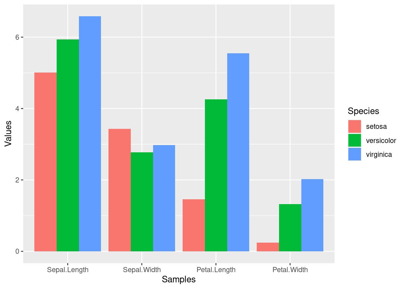
Example 3
Combining dplyr chaining with ggplot
iris_df %>%
    group_by(Species) %>%
    summarize_all(mean) %>%
    reshape2::melt(id.vars=c("Species"), variable.name = "Samples", value.name="Values") %>%
    ggplot(aes(Samples, Values, fill = Species)) +
            geom_bar(position="dodge", stat="identity")
SQLite Databases
SQLite is a lightweight relational database solution. The RSQLite package provides an easy to use interface to create, manage and query SQLite databases directly from R. Basic instructions
for using SQLite from the command-line are available here. A short introduction to RSQLite is available here.
Loading data into SQLite databases
The following loads two data.frames derived from the iris data set (here mydf1 and mydf2)
into an SQLite database (here test.db).
library(RSQLite)
unlink("test.db") # Delete any existing test.db
mydb <- dbConnect(SQLite(), "test.db") # Creates database file test.db
mydf1 <- data.frame(ids=paste0("id", seq_along(iris[,1])), iris)
mydf2 <- mydf1[sample(seq_along(mydf1[,1]), 10),]
dbWriteTable(mydb, "mydf1", mydf1)
dbWriteTable(mydb, "mydf2", mydf2)
List names of tables in database
dbListTables(mydb)
## [1] "mydf1" "mydf2"
Import table into data.frame
dbGetQuery(mydb, 'SELECT * FROM mydf2')
##      ids Sepal.Length Sepal.Width Petal.Length Petal.Width    Species
## 1   id95          5.6         2.7          4.2         1.3 versicolor
## 2   id79          6.0         2.9          4.5         1.5 versicolor
## 3  id124          6.3         2.7          4.9         1.8  virginica
## 4   id33          5.2         4.1          1.5         0.1     setosa
## 5   id48          4.6         3.2          1.4         0.2     setosa
## 6  id122          5.6         2.8          4.9         2.0  virginica
## 7  id104          6.3         2.9          5.6         1.8  virginica
## 8   id56          5.7         2.8          4.5         1.3 versicolor
## 9  id105          6.5         3.0          5.8         2.2  virginica
## 10  id43          4.4         3.2          1.3         0.2     setosa
Query database
dbGetQuery(mydb, 'SELECT * FROM mydf1 WHERE "Sepal.Length" < 4.6')
##    ids Sepal.Length Sepal.Width Petal.Length Petal.Width Species
## 1  id9          4.4         2.9          1.4         0.2  setosa
## 2 id14          4.3         3.0          1.1         0.1  setosa
## 3 id39          4.4         3.0          1.3         0.2  setosa
## 4 id42          4.5         2.3          1.3         0.3  setosa
## 5 id43          4.4         3.2          1.3         0.2  setosa
Join tables
The two tables can be joined on the shared ids column as follows.
dbGetQuery(mydb, 'SELECT * FROM mydf1, mydf2 WHERE mydf1.ids = mydf2.ids')
##      ids Sepal.Length Sepal.Width Petal.Length Petal.Width    Species   ids Sepal.Length
## 1   id33          5.2         4.1          1.5         0.1     setosa  id33          5.2
## 2   id43          4.4         3.2          1.3         0.2     setosa  id43          4.4
## 3   id48          4.6         3.2          1.4         0.2     setosa  id48          4.6
## 4   id56          5.7         2.8          4.5         1.3 versicolor  id56          5.7
## 5   id79          6.0         2.9          4.5         1.5 versicolor  id79          6.0
## 6   id95          5.6         2.7          4.2         1.3 versicolor  id95          5.6
## 7  id104          6.3         2.9          5.6         1.8  virginica id104          6.3
## 8  id105          6.5         3.0          5.8         2.2  virginica id105          6.5
## 9  id122          5.6         2.8          4.9         2.0  virginica id122          5.6
## 10 id124          6.3         2.7          4.9         1.8  virginica id124          6.3
##    Sepal.Width Petal.Length Petal.Width    Species
## 1          4.1          1.5         0.1     setosa
## 2          3.2          1.3         0.2     setosa
## 3          3.2          1.4         0.2     setosa
## 4          2.8          4.5         1.3 versicolor
## 5          2.9          4.5         1.5 versicolor
## 6          2.7          4.2         1.3 versicolor
## 7          2.9          5.6         1.8  virginica
## 8          3.0          5.8         2.2  virginica
## 9          2.8          4.9         2.0  virginica
## 10         2.7          4.9         1.8  virginica
Session Info
sessionInfo()
## R version 4.2.0 (2022-04-22)
## Platform: x86_64-pc-linux-gnu (64-bit)
## Running under: Debian GNU/Linux 11 (bullseye)
##
## Matrix products: default
## BLAS:   /usr/lib/x86_64-linux-gnu/blas/libblas.so.3.9.0
## LAPACK: /usr/lib/x86_64-linux-gnu/lapack/liblapack.so.3.9.0
##
## locale:
##  [1] LC_CTYPE=en_US.UTF-8       LC_NUMERIC=C               LC_TIME=en_US.UTF-8
##  [4] LC_COLLATE=en_US.UTF-8     LC_MONETARY=en_US.UTF-8    LC_MESSAGES=en_US.UTF-8
##  [7] LC_PAPER=en_US.UTF-8       LC_NAME=C                  LC_ADDRESS=C
## [10] LC_TELEPHONE=C             LC_MEASUREMENT=en_US.UTF-8 LC_IDENTIFICATION=C
##
## attached base packages:
## [1] stats     graphics  grDevices utils     datasets  methods   base
##
## other attached packages:
##  [1] RSQLite_2.2.14    data.table_1.14.2 forcats_0.5.1     stringr_1.4.0     dplyr_1.0.9
##  [6] purrr_0.3.4       readr_2.1.2       tidyr_1.2.0       tibble_3.1.7      tidyverse_1.3.1
## [11] ggplot2_3.3.6     limma_3.52.0      BiocStyle_2.24.0
##
## loaded via a namespace (and not attached):
##  [1] Rcpp_1.0.8.3        lubridate_1.8.0     assertthat_0.2.1    digest_0.6.29
##  [5] utf8_1.2.2          plyr_1.8.7          R6_2.5.1            cellranger_1.1.0
##  [9] backports_1.4.1     reprex_2.0.1        evaluate_0.15       highr_0.9
## [13] httr_1.4.3          pillar_1.7.0        rlang_1.0.2         readxl_1.4.0
## [17] rstudioapi_0.13     blob_1.2.3          jquerylib_0.1.4     rmarkdown_2.14
## [21] labeling_0.4.2      bit_4.0.4           munsell_0.5.0       broom_0.8.0
## [25] compiler_4.2.0      modelr_0.1.8        xfun_0.30           pkgconfig_2.0.3
## [29] htmltools_0.5.2     tidyselect_1.1.2    codetools_0.2-18    fansi_1.0.3
## [33] crayon_1.5.1        tzdb_0.3.0          dbplyr_2.1.1        withr_2.5.0
## [37] grid_4.2.0          jsonlite_1.8.0      gtable_0.3.0        lifecycle_1.0.1
## [41] DBI_1.1.2           magrittr_2.0.3      scales_1.2.0        cachem_1.0.6
## [45] cli_3.3.0           stringi_1.7.6       vroom_1.5.7         farver_2.1.0
## [49] reshape2_1.4.4      fs_1.5.2            xml2_1.3.3          bslib_0.3.1
## [53] ellipsis_0.3.2      generics_0.1.2      vctrs_0.4.1         tools_4.2.0
## [57] bit64_4.0.5         glue_1.6.2          hms_1.1.1           parallel_4.2.0
## [61] fastmap_1.1.0       yaml_2.3.5          colorspace_2.0-3    BiocManager_1.30.17
## [65] rvest_1.0.2         memoise_2.0.1       knitr_1.39          haven_2.5.0
## [69] sass_0.4.1