systemPipeR: Workflow Design and Reporting Environment

35 minute read

Introduction

systemPipeR provides flexible utilities for designing, building and running automated end-to-end analysis workflows for a wide range of research applications, including next-generation sequencing (NGS) experiments, such as RNA-Seq, ChIP-Seq, VAR-Seq and Ribo-Seq (H Backman and Girke 2016). Important features include a uniform workflow interface across different data analysis applications, automated report generation, and support for running both R and command-line software, such as NGS aligners or peak/variant callers, on local computers or compute clusters (Figure 1). The latter supports interactive job submissions and batch submissions to queuing systems of clusters.

systemPipeR has been designed to improve the reproducibility of large-scale data analysis projects while substantially reducing the time it takes to analyze complex omics data sets. It provides a uniform workflow interface and management system that allows the users to run selected workflow steps, as well as customize and design entirely new workflows. Additionally, the package take advantage of central community S4 classes of the Bioconductor ecosystem, and enhances them with command-line software support.

The main motivation and advantages of using systemPipeR for complex data analysis tasks are:

1. Design of complex workflows involving multiple R/Bioconductor packages
2. Common workflow interface for different applications
3. User-friendly access to widely used Bioconductor utilities
4. Support of command-line software from within R
5. Reduced complexity of using compute clusters from R
6. Accelerated runtime of workflows via parallelization on computer systems with multiple CPU cores and/or multiple nodes
7. Improved reproducibility by automating the generation of analysis reports

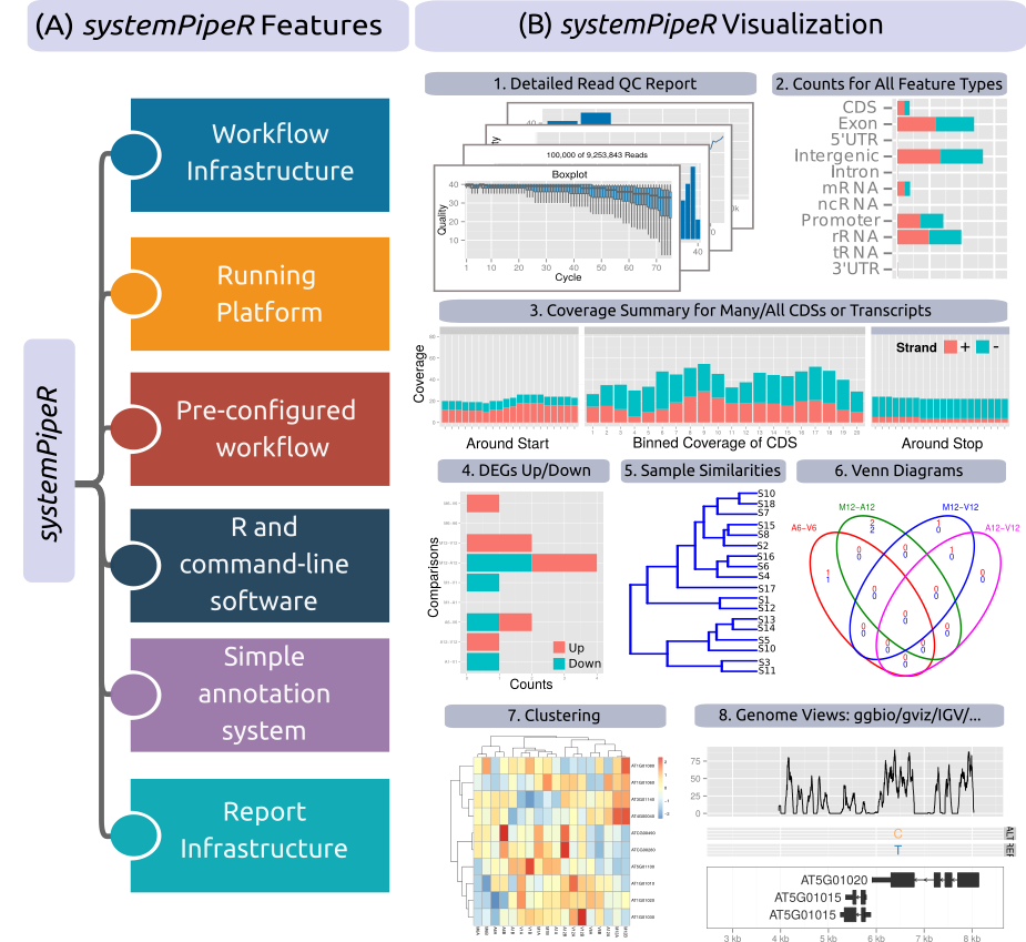
Figure 1: Relevant features in systemPipeR. Workflow design concepts are illustrated under (A). Examples of systemPipeR's visualization functionalities are given under (B).

A central concept for designing workflows within the systemPipeR environment is the use of workflow management containers. Workflow management containers facilitate the design and execution of complex data analysis steps. For its command-line interface systemPipeR adopts the widely used Common Workflow Language (CWL) (Amstutz et al. 2016). The interface to CWL is established by systemPipeR's workflow control class called SYSargsList (see Figure 2). This design offers many advantages such as: (i) options to run workflows either entirely from within R, from various command-line wrappers (e.g., cwl-runner) or from other languages (e.g., Bash or Python). Apart from providing support for both command-line and R/Bioconductor software, the package provides utilities for containerization, parallel evaluations on computer clusters and automated generation of interactive analysis reports.

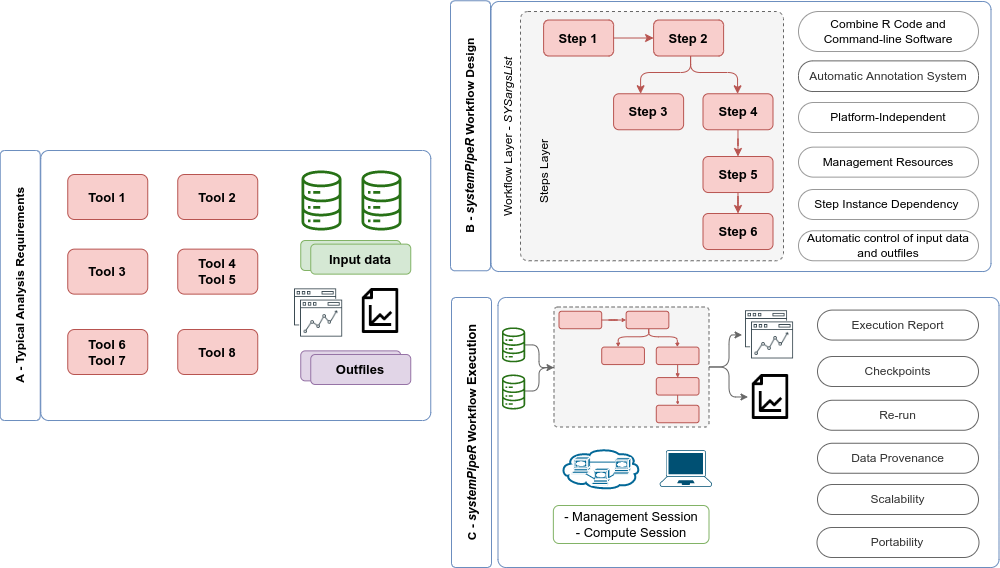
Figure 2: Overview of systemPipeR workflows management instances. (A) A typical analysis workflow requires multiple software tools (red), as well the description of the input (green) and output files, including analysis reports (purple). (B) systemPipeR provides multiple utilities to design and build a workflow, allowing multi-instance, integration of R code and command-line software, a simple and efficient annotation system, that allows automatic control of the input and output data, and multiple resources to manage the entire workflow. (C) Options are provided to execute single or multiple workflow steps, while enabling scalability, checkpoints, and generation of technical and scientific reports.

An important feature of systemPipeR's CWL interface is that it provides two options to run command-line tools and workflows based on CWL. First, one can run CWL in its native way via an R-based wrapper utility for cwl-runner or cwl-tools (CWL-based approach). Second, one can run workflows using CWL’s command-line and workflow instructions from within R (R-based approach). In the latter case the same CWL workflow definition files (e.g. *.cwl and *.yml) are used but rendered and executed entirely with R functions defined by systemPipeR, and thus use CWL mainly as a command-line and workflow definition format rather than execution software to run workflows. In this regard systemPipeR also provides several convenience functions that are useful for designing and debugging workflows, such as a command-line rendering function to retrieve the exact command-line strings for each data set and processing step prior to running a command-line.

Workflow Management with SYSargsList

The SYSargsList S4 class is a list-like container that stores the paths to all input and output files along with the corresponding parameters used in each analysis step (see Figure 3). SYSargsList instances are constructed from an optional targets files, and two CWL parameter files including *.cwl and *.yml (for details, see below). When running preconfigured NGS workflows, the only input the user needs to provide is the initial targets file containing the paths to the input files (e.g., FASTQ) and experiment design information, such as sample labels and biological replicates. Subsequent targets instances are created automatically, based on the connectivity establish between each workflow step. SYSargsList containers store all information required for one or multiple steps. This establishes central control for running, monitoring and debugging complex workflows from start to finish.

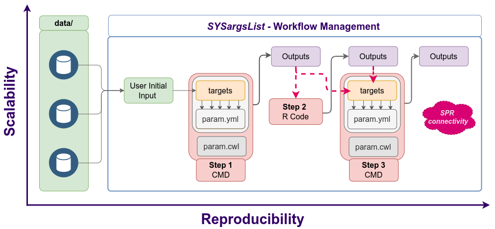
Figure 3: Workflow steps with input/output file operations are controlled by the SYSargsList container. Each of its components (SYSargs2) are constructed from an optional targets and two param files. Alternatively, LineWise instances containing pure R code can be used.

Getting Started

Installation

The R software for running systemPipeR can be downloaded from CRAN. The systemPipeR environment can be installed from the R console using the BiocManager::install command. The associated data package systemPipeRdata can be installed the same way. The latter is a helper package for generating systemPipeR workflow environments with a single command containing all parameter files and sample data required to quickly test and run workflows.

if (!requireNamespace("BiocManager", quietly = TRUE)) install.packages("BiocManager")
BiocManager::install("systemPipeR")
BiocManager::install("systemPipeRdata")

To use command-line software, the corresponding tool and dependencies need to be installed on a user’s system. See details.

Loading package and documentation

library("systemPipeR")  # Loads the package
library(help = "systemPipeR")  # Lists package info
vignette("systemPipeR")  # Opens vignette

Load sample data and workflow templates

The mini sample FASTQ files used by this introduction as well as the associated workflow reporting vignettes can be loaded via the systemPipeRdata package as shown below. The chosen data set SRP010938 contains 18 paired-end (PE) read sets from Arabidposis thaliana (Howard et al. 2013). To minimize processing time during testing, each FASTQ file has been subsetted to 90,000-100,000 randomly sampled PE reads that map to the first 100,000 nucleotides of each chromosome of the A. thalina genome. The corresponding reference genome sequence (FASTA) and its GFF annotation files (provided in the same download) have been truncated accordingly. This way the entire test sample data set requires less than 200MB disk storage space. A PE read set has been chosen for this test data set for flexibility, because it can be used for testing both types of analysis routines requiring either SE (single-end) reads or PE reads.

The following generates a fully populated systemPipeR workflow environment (here for RNA-Seq) in the current working directory of an R session. The systemPipeRdata package provides preconfigured workflow templates for RNA-Seq, ChIP-Seq, VAR-Seq, and Ribo-Seq. Additional, templates are available on the project web site here.

systemPipeRdata::genWorkenvir(workflow = "rnaseq")
setwd("rnaseq")

Project structure

The working environment of the sample data loaded in the previous step contains the following pre-configured directory structure (Figure 4). Directory names are indicated in green. Users can change this structure as needed, but need to adjust the code in their workflows accordingly.

• workflow/ (e.g. rnaseq/)
  • This is the root directory of the R session running the workflow.
  • Run script ( *.Rmd) and sample annotation (targets.txt) files are located here.
  • Note, this directory can have any name (e.g. rnaseq, varseq). Changing its name does not require any modifications in the run script(s).
  • Important subdirectories:
    • param/
      • param/cwl/: This subdirectory stores all the CWL parameter files. To organize workflows, each can have its own subdirectory, where all CWL param and input.yml files need to be in the same subdirectory.
    • data/
      • FASTQ files
      • FASTA file of reference (e.g. reference genome)
      • Annotation files
      • etc.
    • results/
      • Analysis results are usually written to this directory, including: alignment, variant and peak files (BAM, VCF, BED); tabular result files; and image/plot files.
      • Note, the user has the option to organize results files for a given sample and analysis step in a separate subdirectory.

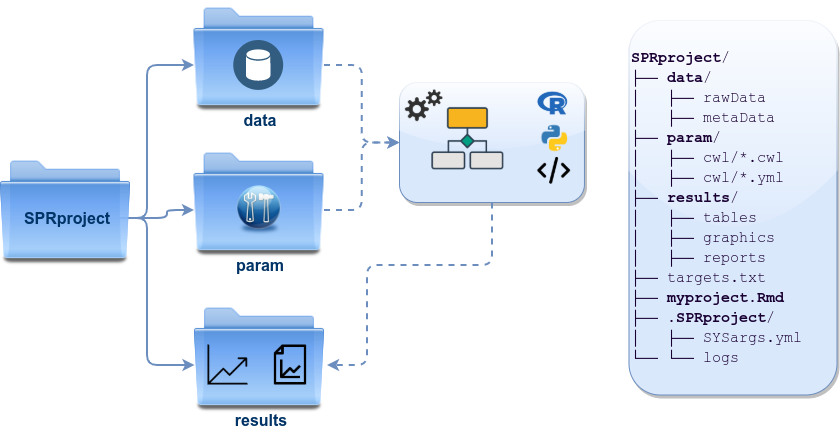
Figure 4: systemPipeR’s preconfigured directory structure.

The following parameter files are included in each workflow template:

1. targets.txt: initial one provided by user; downstream targets_*.txt files are generated automatically
2. *.param/cwl: defines parameter for input/output file operations, e.g.:
   • hisat2/hisat2-mapping-se.cwl
   • hisat2/hisat2-mapping-se.yml
3. Configuration files for computer cluster environments (skip on single machines):
   • .batchtools.conf.R: defines the type of scheduler for batchtools pointing to template file of cluster, and located in user’s home directory
   • *.tmpl: specifies parameters of scheduler used by a system, e.g. Torque, SGE, Slurm, etc.

Structure of targets file

The targets file defines all input files (e.g. FASTQ, BAM, BCF) and sample comparisons of an analysis workflow. The following shows the format of a sample targets file included in the package. It also can be viewed and downloaded from systemPipeR’s GitHub repository here. In a target file with a single type of input files, here FASTQ files of single-end (SE) reads, the first three columns are mandatory including their column names, while it is four mandatory columns for FASTQ files of PE reads. All subsequent columns are optional and any number of additional columns can be added as needed. The columns in targets files are expected to be tab separated (TSV format). The SampleName column contains usually short labels for referencing samples (here FASTQ files) across many workflow steps (e.g. plots and column titles). Importantly, the labels used in the SampleName column need to be unique, while technical or biological replicates are indicated by duplicated values under the Factor column. For readability and transparency, it is useful to use here a short, consistent and informative syntax for naming samples and replicates. To avoid problems with other packages or external software, it is recommended to use the basic naming rules for R objects and their components as outlined here. This is important since the values used under the SampleName and Factor columns are intended to be used as labels for naming columns or plotting features in downstream analysis steps.

Users should note here, the usage of targets files is optional when using systemPipeR’s new CWL interface. They can be replaced by a standard YAML input file used by CWL. Since for organizing experimental variables targets files are extremely useful and user-friendly. Thus, we encourage users to keep using them.

Structure of targets file for single-end (SE) samples

library(systemPipeR)
targetspath <- system.file("extdata", "targets.txt", package = "systemPipeR")
showDF(read.delim(targetspath, comment.char = "#"))

To work with custom data, users need to generate a targets file containing the paths to their own FASTQ files and then provide under targetspath the path to the corresponding targets file.

Structure of targets file for paired-end (PE) samples

For paired-end (PE) samples, the structure of the targets file is similar, where users need to provide two FASTQ path columns: FileName1 and FileName2 with the paths to the PE FASTQ files.

targetspath <- system.file("extdata", "targetsPE.txt", package = "systemPipeR")
showDF(read.delim(targetspath, comment.char = "#"))

Sample comparisons

Sample comparisons are defined in the header lines of the targets file starting with ‘# <CMP>’.

readLines(targetspath)[1:4]

## [1] "# Project ID: Arabidopsis - Pseudomonas alternative splicing study (SRA: SRP010938; PMID: 24098335)"                                                                              
## [2] "# The following line(s) allow to specify the contrasts needed for comparative analyses, such as DEG identification. All possible comparisons can be specified with 'CMPset: ALL'."
## [3] "# <CMP> CMPset1: M1-A1, M1-V1, A1-V1, M6-A6, M6-V6, A6-V6, M12-A12, M12-V12, A12-V12"                                                                                             
## [4] "# <CMP> CMPset2: ALL"

The function readComp imports the comparison information and stores it in a list. Alternatively, readComp can obtain the comparison information from the corresponding SYSargsList object (see below). Note, these header lines are optional. They are mainly useful for controlling comparative analyses according to certain biological expectations, such as identifying differentially expressed genes in RNA-Seq experiments based on simple pair-wise comparisons.

readComp(file = targetspath, format = "vector", delim = "-")

## $CMPset1
## [1] "M1-A1"   "M1-V1"   "A1-V1"   "M6-A6"   "M6-V6"   "A6-V6"   "M12-A12"
## [8] "M12-V12" "A12-V12"
## 
## $CMPset2
##  [1] "M1-A1"   "M1-V1"   "M1-M6"   "M1-A6"   "M1-V6"   "M1-M12"  "M1-A12" 
##  [8] "M1-V12"  "A1-V1"   "A1-M6"   "A1-A6"   "A1-V6"   "A1-M12"  "A1-A12" 
## [15] "A1-V12"  "V1-M6"   "V1-A6"   "V1-V6"   "V1-M12"  "V1-A12"  "V1-V12" 
## [22] "M6-A6"   "M6-V6"   "M6-M12"  "M6-A12"  "M6-V12"  "A6-V6"   "A6-M12" 
## [29] "A6-A12"  "A6-V12"  "V6-M12"  "V6-A12"  "V6-V12"  "M12-A12" "M12-V12"
## [36] "A12-V12"

Project initialization

To create a workflow within systemPipeR, we can start by defining an empty container and checking the directory structure:

sal <- SPRproject()

## Creating directory '/home/tgirke/tmp/GEN242/content/en/tutorials/systempiper/rnaseq/.SPRproject'
## Creating file '/home/tgirke/tmp/GEN242/content/en/tutorials/systempiper/rnaseq/.SPRproject/SYSargsList.yml'

Internally, SPRproject function will create a hidden directory called .SPRproject, by default. This directory will store all log files generated during a workflow run.

Initially, the object sal is a empty container containing only the basic project information. The project information can be accessed with the projectInfo method.

sal

## Instance of 'SYSargsList': 
##  No workflow steps added

projectInfo(sal)

## $project
## [1] "/home/tgirke/tmp/GEN242/content/en/tutorials/systempiper/rnaseq"
## 
## $data
## [1] "data"
## 
## $param
## [1] "param"
## 
## $results
## [1] "results"
## 
## $logsDir
## [1] ".SPRproject"
## 
## $sysargslist
## [1] ".SPRproject/SYSargsList.yml"

Also, the length function will return how many steps a workflow contains. Since no steps have been added yet it returns zero.

length(sal)

## [1] 0

Building workflows

systemPipeR workflows can be populated with a single command from an R Markdown file or stepwise in interactive mode. This section introduces first how to build a workflow stepwise in interactive mode, and then how to build a workflow with a single command from an R Markdown file.

Stepwise workflow construction

New workflows are constructed, or existing ones modified, by connecting each step via the appendStep method. Each step in a SYSargsList instance contains the instructions needed for processing a set of input files with a specific command-line and the paths to the exptected outfiles. For constructing R code-based workflow steps the constructor function Linewise is used.

The following demonstrates how to create a command-line workflow step here using as example the short read aligner software HISAT2 (Kim, Langmead, and Salzberg 2015).

The constructor function renders the proper command-line strings for each sample and software tool, appending a new step in the SYSargsList object defined in the previous step. For this, the SYSargsList constructor function uses in this example data from three input files:

• CWL command-line specification file (wf_file argument)
• Input variables (input_file argument)
• Targets file (targets argument)

In CWL files with the extension .cwl define the parameters of a chosen command-line step or an entire workflow, while files with the extension .yml define the input variables of command-line steps. Note, input variables provided by a targets or targetsPE file can be passed on via the inputvars argument to the .yml file and from there to the SYSargsList object.

appendStep(sal) <- SYSargsList(step_name = "hisat2_mapping", dir = TRUE, targets = "targetsPE.txt",
    wf_file = "workflow-hisat2/workflow_hisat2-pe.cwl", input_file = "workflow-hisat2/workflow_hisat2-pe.yml",
    dir_path = "param/cwl", inputvars = c(FileName1 = "_FASTQ_PATH1_", FileName2 = "_FASTQ_PATH2_",
        SampleName = "_SampleName_"))

An overview of the workflow can be printed as follows.

sal

## Instance of 'SYSargsList': 
##     WF Steps:
##        1. hisat2_mapping --> Status: Pending 
##            Total Files: 72 | Existing: 0 | Missing: 72 
##          1.1. hisat2
##              cmdlist: 18 | Pending: 18
##          1.2. samtools-view
##              cmdlist: 18 | Pending: 18
##          1.3. samtools-sort
##              cmdlist: 18 | Pending: 18
##          1.4. samtools-index
##              cmdlist: 18 | Pending: 18
## 

In the above the workflow status for the new step is Pending. This means the workflow object has been constructed but not executed yet.

Several accessor methods are available to explore the SYSargsList object. Of particular interest is the cmdlist() method. It constructs the system commands for running command-line software as specified by a given .cwl file combined with the paths to the input samples (e.g. FASTQ files), here provided by a targets file. The example below shows the cmdlist() output for running HISAT2 on the first PE read sample. Evaluating the output of cmdlist() can be very helpful for designing and debugging .cwl files of new command-line software or changing the parameter settings of existing ones. The rendered command-line instance for each input sample can be returned as follows.

cmdlist(sal, step = "hisat2_mapping", targets = 1)

## $hisat2_mapping
## $hisat2_mapping$M1A
## $hisat2_mapping$M1A$hisat2
## [1] "hisat2 -S ./results/M1A.sam  -x ./data/tair10.fasta  -k 1  --min-intronlen 30  --max-intronlen 3000  -1 ./data/SRR446027_1.fastq.gz -2 ./data/SRR446027_2.fastq.gz --threads 4"
## 
## $hisat2_mapping$M1A$`samtools-view`
## [1] "samtools view -bS -o ./results/M1A.bam  ./results/M1A.sam "
## 
## $hisat2_mapping$M1A$`samtools-sort`
## [1] "samtools sort -o ./results/M1A.sorted.bam  ./results/M1A.bam  -@ 4"
## 
## $hisat2_mapping$M1A$`samtools-index`
## [1] "samtools index -b results/M1A.sorted.bam  results/M1A.sorted.bam.bai  ./results/M1A.sorted.bam "

The outfiles components of SYSargsList define the expected output files for each step in the workflow; some of which are the input for the next workflow step (see Figure 3).

outfiles(sal)

## $hisat2_mapping
## DataFrame with 18 rows and 4 columns
##              hisat2_sam       samtools_bam      samtools_sort_bam
##             <character>        <character>            <character>
## M1A   ./results/M1A.sam  ./results/M1A.bam ./results/M1A.sorted..
## M1B   ./results/M1B.sam  ./results/M1B.bam ./results/M1B.sorted..
## A1A   ./results/A1A.sam  ./results/A1A.bam ./results/A1A.sorted..
## A1B   ./results/A1B.sam  ./results/A1B.bam ./results/A1B.sorted..
## V1A   ./results/V1A.sam  ./results/V1A.bam ./results/V1A.sorted..
## ...                 ...                ...                    ...
## M12B ./results/M12B.sam ./results/M12B.bam ./results/M12B.sorte..
## A12A ./results/A12A.sam ./results/A12A.bam ./results/A12A.sorte..
## A12B ./results/A12B.sam ./results/A12B.bam ./results/A12B.sorte..
## V12A ./results/V12A.sam ./results/V12A.bam ./results/V12A.sorte..
## V12B ./results/V12B.sam ./results/V12B.bam ./results/V12B.sorte..
##              samtools_index
##                 <character>
## M1A  ./results/M1A.sorted..
## M1B  ./results/M1B.sorted..
## A1A  ./results/A1A.sorted..
## A1B  ./results/A1B.sorted..
## V1A  ./results/V1A.sorted..
## ...                     ...
## M12B ./results/M12B.sorte..
## A12A ./results/A12A.sorte..
## A12B ./results/A12B.sorte..
## V12A ./results/V12A.sorte..
## V12B ./results/V12B.sorte..

In an ‘R-centric’ rather than a ‘CWL-centric’ workflow design the connectivity among workflow steps is established by creating the downstream targets instances automatically (see Figure 3). Each step uses the outfiles from the previous step as input, thereby establishing connectivity among each step in the workflow. By chaining several SYSargsList steps together one can construct complex workflows involving many sample-level input/output file operations with any combination of command-line or R-based software. Also, systemPipeR provides features to automatically build these connections. This provides additional security to make sure that all samples will be processed in a reproducible manner.

Alternatively, a CWL-centric workflow design can be used that defines all or most workflow steps with CWL workflow and parameter files. Due to time and space restrictions, the CWL-centric approach is not covered by this tutorial.

The following R code step generates a data.frame containing important read alignment statistics such as the total number of reads in the FASTQ files, the number of total alignments, as well as the number of primary alignments in the corresponding BAM files. The constructor function LineWise requires the step_name and the R code assigned to the code argument. The R code should be enclosed by braces ({}).

appendStep(sal) <- LineWise(code = {
    fqpaths <- getColumn(sal, step = "hisat2_mapping", "targetsWF", column = "FileName1")
    bampaths <- getColumn(sal, step = "hisat2_mapping", "outfiles", column = "samtools_sort_bam")
    read_statsDF <- alignStats(args = bampaths, fqpaths = fqpaths, pairEnd = TRUE)
    write.table(read_statsDF, "results/alignStats.xls", row.names = FALSE, quote = FALSE,
        sep = "\t")
}, step_name = "align_stats", dependency = "hisat2_mapping")

To inspect the R code of this step, the codeLine method can be used.

codeLine(sal, "align_stats")

## align_stats
##     fqpaths <- getColumn(sal, step = "hisat2_mapping", "targetsWF", column = "FileName1")
##     bampaths <- getColumn(sal, step = "hisat2_mapping", "outfiles", column = "samtools_sort_bam")
##     read_statsDF <- alignStats(args = bampaths, fqpaths = fqpaths, pairEnd = TRUE)
##     write.table(read_statsDF, "results/alignStats.xls", row.names = FALSE, quote = FALSE, sep = "\t")

The getColumn method allows to extract certain information of a workflow instance, here output files that can be accessed from within R as demonstrated below.

getColumn(sal, step = "hisat2_mapping", "outfiles", column = "samtools_sort_bam")

##                         M1A                         M1B 
##  "./results/M1A.sorted.bam"  "./results/M1B.sorted.bam" 
##                         A1A                         A1B 
##  "./results/A1A.sorted.bam"  "./results/A1B.sorted.bam" 
##                         V1A                         V1B 
##  "./results/V1A.sorted.bam"  "./results/V1B.sorted.bam" 
##                         M6A                         M6B 
##  "./results/M6A.sorted.bam"  "./results/M6B.sorted.bam" 
##                         A6A                         A6B 
##  "./results/A6A.sorted.bam"  "./results/A6B.sorted.bam" 
##                         V6A                         V6B 
##  "./results/V6A.sorted.bam"  "./results/V6B.sorted.bam" 
##                        M12A                        M12B 
## "./results/M12A.sorted.bam" "./results/M12B.sorted.bam" 
##                        A12A                        A12B 
## "./results/A12A.sorted.bam" "./results/A12B.sorted.bam" 
##                        V12A                        V12B 
## "./results/V12A.sorted.bam" "./results/V12B.sorted.bam"

Loading workflows from an R Markdown

The importWF function allows to load an entire workflow from an R Markdown (Rmd) file into an SYSargsList object that has been intialized with SPRproject() as introduced above. Next, one can run the workflow from start to finish with a single function call using runWF. Below the latter has been commented out to first introduce additional details prior to executing the workflow with runWF, which will be discussed in the following section.

sal <- SPRproject()

## Creating directory '/home/tgirke/tmp/GEN242/content/en/tutorials/systempiper/rnaseq/.SPRproject'
## Creating file '/home/tgirke/tmp/GEN242/content/en/tutorials/systempiper/rnaseq/.SPRproject/SYSargsList.yml'

sal <- importWF(sal, file_path = "systemPipeRNAseq.Rmd")

## Reading Rmd file

## 
##  ---- Actions ----

## Ignore none-R chunks at line: 25

## Checking chunk eval values

## Checking chunk SPR option

## Ignore non-SPR chunks: 34, 43, 61, 96, 121, 188, 205, 298, 658, 686, 704, 712, 723

## Parse chunk code

## Now importing step 'load_SPR' 
## Now importing step 'preprocessing' 
## Now importing step 'trimming' 
## Now importing step 'fastq_report' 
## Now importing step 'hisat2_index' 
## Now importing step 'hisat2_mapping' 
## Now importing step 'align_stats' 
## Now importing step 'bam_IGV' 
## Now importing step 'create_db' 
## Now importing step 'read_counting' 
## Now importing step 'sample_tree' 
## Now importing step 'run_edger' 
## Now importing step 'custom_annot' 
## Now importing step 'filter_degs' 
## Now importing step 'venn_diagram' 
## Now importing step 'get_go_annot' 
## Now importing step 'go_enrich' 
## Now importing step 'go_plot' 
## Now importing step 'heatmap' 
## Now importing step 'sessionInfo'

# sal <- runWF(sal)

Several accessor functions are available to inspect the workflow.

stepsWF(sal)
dependency(sal)
codeLine(sal)
targetsWF(sal)

Third-party software tools

Examples of preconfigured CWL templates for third-party software tools are provided in the following table. In addition, the tutorial entitled Automate Creation of CWL Instructions explains how to create these CWL templates for essentially any command-line tool simply by providing the command-line string for a new software as input.

Importantly, command-line software needs to be installed on a user’s system
and available in a user’s PATH. To check whether this is the case, one can use the
tryCL function.

tryCL(command = "grep")

How to run workflows?

Setup and requirements

To execute the code in this tutorial, one needs the following software installed.

• R (version >=4.1.2)
• systemPipeR package (version >=2.0.8)
• Hisat2 (version >= 2.1.0)

To build custom workflows with any additional command-line software, one needs the respective software installed and available in the user PATH. To test this, one can use the tryCL function.

tryCL(command = "hisat2")  ## 'All set up, proceed!'

Run from R

For running a workflow, the runWF function can be used. It executes all workflow steps stored in a SYSargsList container (below named sal). This assumes the sal object has been initialized and populated as outlined above using SPRproject() and importWF(sal, file_path="..."), respectively.

sal <- runWF(sal)

This essential function allows the user to choose one or multiple steps to be executed using its steps argument. However, it is necessary to maintain valid dependencies (also see workflow graph). If a selected step depends on a previous step(s), the output of which may not be available yet, then the execution will fail.

sal <- runWF(sal, steps = c(1, 3))

The runWF function allows to force the execution of chosen workflow steps, even if the status of a given step is 'Success' and the expected outfiles exist already. This is useful for updating certain steps when needed. Another option is to force runWF to ignore all warnings and errors. This can be achieved by assigning FALSE to the arguments warning.stop and error.stop, respectively.

sal <- runWF(sal, force = TRUE, warning.stop = FALSE, error.stop = FALSE)

While SYSargsList (sal) objects are autosaved when working with workflows, it can be sometimes safer to explicity save the object before closing R.

sal <- write_SYSargsList(sal)

Resume and reset workflows

To restart workflows, set resume=TRUE.

sal <- SPRproject(resume = TRUE)

To delete all steps in a workflow including the content saved under the .SPRproject directory, use overwrite=TRUE. This option should be used with caution, since it effectively deletes most previous workflow data.

sal <- SPRproject(overwrite = TRUE)

For additional options and details, users want to consult the help documentation for: ?SPRproject, ?runWF and ?'SYSargsList-class'.

Parallelization on clusters

The computation of time-consuming steps can be greatly accelerated by processing many files in parallel using several compute nodes of a cluster, where a scheduling system is used for load balancing.

The following resources list provides to a SYSargsList (sal) object the number of independent parallel cluster processes defined under the Njobs element in the list. The given example will run 18 processes in parallel using for each 4 CPU cores, thus utilizing a total of 72 CPU cores. Note, runWF can be used with most queueing systems as it is based on utilities defined by the batchtools package, which supports the use of template files (*.tmpl) for defining the run parameters of different schedulers. To run the following code, one needs to have both a conffile (see .batchtools.conf.R samples here) and a template file (see *.tmpl samples here) for the queueing system available on a system. The following example uses the sample conffile and template files for the Slurm scheduler provided by this package.

The resources list can be appended when a workflow step is generated. Alternatively, one can append these resource specifications to any step of a pre-generated SYSarsList with the addResources function.

resources <- list(conffile=".batchtools.conf.R",
                  template="batchtools.slurm.tmpl", 
                  Njobs=18, 
                  walltime=120, # in min
                  ntasks=1,
                  ncpus=4, 
                  memory=1024, # in Mb
                  partition = "short"  
                  )
sal <- addResources(sal, c("hisat2_mapping"), resources = resources)
sal <- runWF(sal)

The above example will submit via runWF(sal) the hisat2_mapping step to a partition called short on a computer cluster. Users need to adjust this and other parameters defined in the resources list to their environment.

Run from Command-Line (without cluster)

Create an R script containing the following (or similar) minimum content.

#!/usr/bin/env Rscript

library(systemPipeR)
sal <- SPRproject()
sal <- importWF(sal, file_path = "systemPipeRNAseq.Rmd") # adjust name of Rmd file if different  
sal <- runWF(sal) # runs entire workflow
sal <- renderReport(sal) # after workflow has completed render Rmd to HTML report

Assuming the script is named wf_run_script.R it can be executed from the command-line (not R console!) as follows. In addition, one can make the script executable to run it like any other script.

Rscript wf_run_script.R

This will run systemPipeR workflows on a single machine. In this case a limited amount of parallelization is possible if the corresponding code chunks in the workflow take advantage of multi-core parallelization instructions provided by BiocParallel, batchtools or related packages. However, this type of parallelization is usually limited to the number of cores available on a single CPU. A much more scalable approach is the use of computer clusters as described above and in the next section.

Submit workflow from command-line to cluster

In addition to running workflows within interactive R sessions or submitting them from the command-line on a single system (see above), one can execute systemPipeR workflows from the command-line to an HPC cluster by including the relevant workflow run instructions in an R script and then submitting it via a submission script of a workload manager system to a computer cluster. The following gives an example for the Slurm workload manager. To understand the details, it is important to inspect the content of the two files (here .R and .sh). Additional details about resource specification under Slurm are given below.

• R script: wf_run_script.R
• Slurm submission script: wf_run_script.sh

As a test, users can generate in their user account of a cluster a workflow environment populated with the toy data as outlined here. After this, it is best to create within the workflow directory a subdirectory, e.g. called cl_sbatch_run, and then save the above two files to this subdirectory. Next, the parameters in both files need to be adjusted to match the type of workflow and the required computing resources. This includes the name of the Rmd file and scheduler resource settings such as: partition, Njobs, walltime, memory, etc. After all relevant settings have been set correctly, one can execute the workflow with sbatch from within the cl_sbatch_run directory as follows (note this is a command-line call outside of R):

sbatch wf_run_script.sh

After the submission to the cluster, one usually should check its status and progress with squeue -u <username> (under Slurm) as well as by monitoring the content of the slurm-<jobid>.out file generated by the scheduler in the same directory. This file contains most of the STDOUT and STDERROR generated by a cluster job. Once everything is working on the toy data, users can run the workflow on real data the same way.

Visualize workflow

systemPipeR workflows instances can be visualized with the plotWF function. The resulting plot includes the following information.

• Workflow topology graph (dependency graphs between different steps)
• Workflow step status, e.g. Success, Error, Pending, Warnings
• Sample status and statistics
• Workflow timing: run duration time

If no argument is provided, the basic plot will automatically detect width, height, layout, plot method, branches, etc.

plotWF(sal)

Technical reports

systemPipeR compiles all workflow execution logs in one central location, making it easy to check any standard output (stdout) or standard error (stderr) for any command-line tool used in a workflow. Also, the information is appended to the workflow plot making it easy to click on respective steps.

sal <- renderLogs(sal)

Scientific reports

systemPipeR auto-generates scientific analysis reports in HTML format. These reports compile the results of all workflow steps including text, code, plots and tables.

sal <- renderReport(sal)

Alternatively, scientific reports can be rendered with the render function from rmarkdown.

rmarkdown::render("systemPipeRNAseq.Rmd", clean = TRUE, output_format = "BiocStyle::html_document")

How to modify workflows?

Modifying steps

If needed one can modify existing workflow steps in a pre-populated SYSargsList object, and potentially already executed workflows, with the replaceStep(sal) <- replacement function. The following gives an example where step number 3 in a SYSargsList (sal) object will be updated with modified or new code. Note, this is a generalized example where the user needs to insert the code lines between { and }, and also adjust the values assigned to the arguments: step_name and dependency.

replaceStep(sal, step = 3) <- LineWise(code = {
    ...
}, step_name = "my_step_name", dependency = "my_dependency")

Since step_names need to be unique, one should avoid using the same step_name as before. If the previous name is used, a default name will be assigned. Rerunning the assignment will then allow to assign the previous name. This behavior is enforced for version tracking. Subsequently, one can view and check the code changes with codeLine(), and then rerun the corresponding step (here 3) as follows:

codeLine(stepsWF(sal)$my_step_name)
runWF(sal, steps = 3)

As mentioned above, any step in a workflow can only be run in isolation if its expected input exists (see dependency).

Adding steps

New steps can be added to the Rmd file of a workflow by inserting new R Markdown code blocks (chunks) starting and ending with the usual appendStep<- syntax and then creating a new SYSargsList instance with importWF that contain the new step(s). To add steps to a pre-populated SYSargsList object, one can use the after argument of the appendStep<- function. The following example will add a new step after position 3 to the corresponding sal object. This can be useful if a workflow with a long runtime has already been completed and one only wants to make some refinements without re-running the entire workflow.

appendStep(sal, after = 3) <- ...

Workflow templates

Workflow templates are provided via the affiliated Bioconductor data package named systemPipeRdata, as well as by a dedicated GitHub repository. Instances of these workflows can be created with a single command. The following gives several examples.

RNA-Seq WF template

Load the RNA-Seq sample workflow into your current working directory.

library(systemPipeRdata)
genWorkenvir(workflow = "rnaseq")
setwd("rnaseq")

Create the workflow

This template includes the most common analysis steps of RNAseq workflows. One can add, remove, modify workflow steps by modifying the sal object.

sal <- SPRproject()
sal <- importWF(sal, file_path = "systemPipeRNAseq.Rmd", verbose = FALSE)

Workflow steps:

1. Read preprocessing
   • Quality filtering (trimming)
   • FASTQ quality report
2. Alignments: HISAT2 (or any other RNA-Seq aligner)
3. Alignment stats
4. Read counting
5. Sample-wise correlation analysis
6. Analysis of differentially expressed genes (DEGs)
7. GO term enrichment analysis
8. Gene-wise clustering

Run workflow

sal <- runWF(sal)

Workflow visualization

plotWF(sal)

Report generation

sal <- renderReport(sal)
sal <- renderLogs(sal)

ChIP-Seq WF template

Load the ChIP-Seq sample workflow into your current working directory.

library(systemPipeRdata)
genWorkenvir(workflow = "chipseq")
setwd("chipseq")

Workflow steps:

1. Read preprocessing
   • Quality filtering (trimming)
   • FASTQ quality report
2. Alignments: Bowtie2 or rsubread
3. Alignment stats
4. Peak calling: MACS2
5. Peak annotation with genomic context
6. Differential binding analysis
7. GO term enrichment analysis
8. Motif analysis

Create the workflow

This template provides some common steps for a ChIPseq workflow. One can add, remove, modify workflow steps by operating on the sal object.

sal <- SPRproject()
sal <- importWF(sal, file_path = "systemPipeChIPseq.Rmd", verbose = FALSE)

Run workflow

sal <- runWF(sal)

Workflow visualization

plotWF(sal)

Report generation

sal <- renderReport(sal)
sal <- renderLogs(sal)

VAR-Seq WF template

Load the VAR-Seq sample workflow into your current working directory.

library(systemPipeRdata)
genWorkenvir(workflow = "varseq")
setwd("varseq")

Workflow steps:

1. Read preprocessing
   • Quality filtering (trimming)
   • FASTQ quality report
2. Alignments: gsnap, bwa
3. Variant calling: VariantTools, GATK, BCFtools
4. Variant filtering: VariantTools and VariantAnnotation
5. Variant annotation: VariantAnnotation
6. Combine results from many samples
7. Summary statistics of samples

Create the workflow

This template provides some common steps for a VARseq workflow. One can add, remove, modify workflow steps by operating on the sal object.

sal <- SPRproject()
sal <- importWF(sal, file_path = "systemPipeVARseq.Rmd", verbose = FALSE)

Run workflow

sal <- runWF(sal)

Workflow visualization

plotWF(sal)

Report generation

sal <- renderReport(sal)
sal <- renderLogs(sal)

Ribo-Seq WF template

Load the Ribo-Seq sample workflow into your current working directory.

library(systemPipeRdata)
genWorkenvir(workflow = "riboseq")
setwd("riboseq")

Workflow steps:

1. Read preprocessing
   • Adaptor trimming and quality filtering
   • FASTQ quality report
2. Alignments: HISAT2 (or any other RNA-Seq aligner)
3. Alignment stats
4. Compute read distribution across genomic features
5. Adding custom features to workflow (e.g. uORFs)
6. Genomic read coverage along transcripts
7. Read counting
8. Sample-wise correlation analysis
9. Analysis of differentially expressed genes (DEGs)
10. GO term enrichment analysis
11. Gene-wise clustering
12. Differential ribosome binding (translational efficiency)

Create the workflow

This template provides some common steps for a RIBOseq workflow. One can add, remove, modify workflow steps by operating on the sal object.

sal <- SPRproject()
sal <- importWF(sal, file_path = "systemPipeRIBOseq.Rmd", verbose = FALSE)

Run workflow

sal <- runWF(sal)

Workflow visualization

plotWF(sal, rstudio = TRUE)

Report generation

sal <- renderReport(sal)
sal <- renderLogs(sal)

Funding

This project is funded by NSF award ABI-1661152.

Version information

Note: the most recent version of this tutorial can be found here.

sessionInfo()

## R version 4.3.0 (2023-04-21)
## Platform: x86_64-pc-linux-gnu (64-bit)
## Running under: Debian GNU/Linux 11 (bullseye)
## 
## Matrix products: default
## BLAS:   /usr/lib/x86_64-linux-gnu/blas/libblas.so.3.9.0 
## LAPACK: /usr/lib/x86_64-linux-gnu/lapack/liblapack.so.3.9.0
## 
## locale:
##  [1] LC_CTYPE=en_US.UTF-8       LC_NUMERIC=C              
##  [3] LC_TIME=en_US.UTF-8        LC_COLLATE=en_US.UTF-8    
##  [5] LC_MONETARY=en_US.UTF-8    LC_MESSAGES=en_US.UTF-8   
##  [7] LC_PAPER=en_US.UTF-8       LC_NAME=C                 
##  [9] LC_ADDRESS=C               LC_TELEPHONE=C            
## [11] LC_MEASUREMENT=en_US.UTF-8 LC_IDENTIFICATION=C       
## 
## time zone: America/Los_Angeles
## tzcode source: system (glibc)
## 
## attached base packages:
## [1] stats4    stats     graphics  grDevices utils     datasets  methods  
## [8] base     
## 
## other attached packages:
##  [1] magrittr_2.0.3              batchtools_0.9.17          
##  [3] ape_5.7-1                   ggplot2_3.4.2              
##  [5] systemPipeR_2.6.0           ShortRead_1.58.0           
##  [7] GenomicAlignments_1.36.0    SummarizedExperiment_1.30.0
##  [9] Biobase_2.60.0              MatrixGenerics_1.12.0      
## [11] matrixStats_0.63.0          BiocParallel_1.34.0        
## [13] Rsamtools_2.16.0            Biostrings_2.68.0          
## [15] XVector_0.40.0              GenomicRanges_1.52.0       
## [17] GenomeInfoDb_1.36.0         IRanges_2.34.0             
## [19] S4Vectors_0.38.0            BiocGenerics_0.46.0        
## [21] BiocStyle_2.28.0           
## 
## loaded via a namespace (and not attached):
##  [1] tidyselect_1.2.0        dplyr_1.1.2             bitops_1.0-7           
##  [4] fastmap_1.1.1           RCurl_1.98-1.12         blogdown_1.16          
##  [7] digest_0.6.31           base64url_1.4           lifecycle_1.0.3        
## [10] compiler_4.3.0          rlang_1.1.1             sass_0.4.5             
## [13] progress_1.2.2          tools_4.3.0             utf8_1.2.3             
## [16] yaml_2.3.7              data.table_1.14.8       systemPipeRdata_2.4.0  
## [19] knitr_1.42              prettyunits_1.1.1       brew_1.0-8             
## [22] htmlwidgets_1.6.2       interp_1.1-4            DelayedArray_0.25.0    
## [25] RColorBrewer_1.1-3      withr_2.5.0             hwriter_1.3.2.1        
## [28] grid_4.3.0              fansi_1.0.4             latticeExtra_0.6-30    
## [31] colorspace_2.1-0        scales_1.2.1            cli_3.6.1              
## [34] rmarkdown_2.21          crayon_1.5.2            generics_0.1.3         
## [37] remotes_2.4.2           cachem_1.0.7            stringr_1.5.0          
## [40] zlibbioc_1.46.0         parallel_4.3.0          formatR_1.14           
## [43] BiocManager_1.30.20     vctrs_0.6.2             Matrix_1.5-4           
## [46] jsonlite_1.8.4          bookdown_0.33           hms_1.1.3              
## [49] jpeg_0.1-10             jquerylib_0.1.4         glue_1.6.2             
## [52] codetools_0.2-19        stringi_1.7.12          gtable_0.3.3           
## [55] deldir_1.0-6            munsell_0.5.0           tibble_3.2.1           
## [58] pillar_1.9.0            rappdirs_0.3.3          htmltools_0.5.5        
## [61] GenomeInfoDbData_1.2.10 R6_2.5.1                evaluate_0.20          
## [64] lattice_0.21-8          png_0.1-8               backports_1.4.1        
## [67] bslib_0.4.2             Rcpp_1.0.10             nlme_3.1-162           
## [70] checkmate_2.2.0         xfun_0.39               pkgconfig_2.0.3

References

Amstutz, Peter, Michael R Crusoe, Nebojša Tijanić, Brad Chapman, John Chilton, Michael Heuer, Andrey Kartashov, et al. 2016. “Common Workflow Language, V1.0,” July. https://doi.org/10.6084/m9.figshare.3115156.v2.
H Backman, Tyler W, and Thomas Girke. 2016. “systemPipeR: NGS workflow and report generation environment.” BMC Bioinformatics 17 (1): 388. https://doi.org/10.1186/s12859-016-1241-0.
Howard, Brian E, Qiwen Hu, Ahmet Can Babaoglu, Manan Chandra, Monica Borghi, Xiaoping Tan, Luyan He, et al. 2013. “High-Throughput RNA Sequencing of Pseudomonas-Infected Arabidopsis Reveals Hidden Transcriptome Complexity and Novel Splice Variants.” PLoS One 8 (10): e74183. https://doi.org/10.1371/journal.pone.0074183.
Kim, Daehwan, Ben Langmead, and Steven L Salzberg. 2015. “HISAT: A Fast Spliced Aligner with Low Memory Requirements.” Nat. Methods 12 (4): 357–60.