ChIP-Seq Workflow Template
28 minute read
Introduction
Overview
This workflow template is for analyzing ChIP-Seq data. It is provided by
systemPipeRdata,
a companion package to systemPipeR (H Backman and Girke 2016).
Similar to other systemPipeR workflow templates, a single command generates
the necessary working environment. This includes the expected directory
structure for executing systemPipeR workflows and parameter files for running
command-line (CL) software utilized in specific analysis steps. For learning
and testing purposes, a small sample (toy) data set is also included (mainly
FASTQ and reference genome files). This enables users to seamlessly run the
numerous analysis steps of this workflow from start to finish without the
requirement of providing custom data. After testing the workflow, users have
the flexibility to employ the template as is with their own data or modify it
to suit their specific needs. For more comprehensive information on designing
and executing workflows, users want to refer to the main vignettes of
systemPipeR
and
systemPipeRdata.
The Rmd file (systemPipeChIPseq.Rmd) associated with this vignette serves a dual purpose. It acts
both as a template for executing the workflow and as a template for generating
a reproducible scientific analysis report. Thus, users want to customize the text
(and/or code) of this vignette to describe their experimental design and
analysis results. This typically involves deleting the instructions how to work
with this workflow, and customizing the text describing experimental designs,
other metadata and analysis results.
Experimental design
Typically, the user wants to describe here the sources and versions of the
reference genome sequence along with the corresponding annotations. The standard
directory structure of systemPipeR (see here),
expects the input data in a subdirectory named data
and all results will be written to a separate results directory. The Rmd source file
for executing the workflow and rendering its report (here systemPipeChIPseq.Rmd) is
expected to be located in the parent directory.
This workflow template leverages the same test data set as the RNA-Seq workflow within
systemPipeRdata (SRP010938). This data
set comprises 18 paired-end (PE) read sets derived from Arabidopsis thaliana (Howard et al. 2013). By utilizing the
same test data across multiple workflows, the storage footprint of the
systemPipeRdata package is minimized. It is important to note that this approach
does not affect the analysis steps specifically tailored for a ChIP-Seq
analysis workflow. To minimize processing time during testing, each FASTQ file of the test
data set has been reduced to 90,000-100,000 randomly sampled PE reads that map to the first 100,000
nucleotides of each chromosome of the A. thaliana genome. The corresponding
reference genome sequence (FASTA) and its GFF annotation files have been
reduced to the same genome regions. This way the entire test sample data set is
less than 200MB in storage space. A PE read set has been chosen here for
flexibility, because it can be used for testing both types of analysis routines
requiring either SE (single end) reads or PE reads.
To use their own ChIP-Seq and reference genome data, users want to move or link the
data to the designated data directory and execute the workflow from the parent directory
using their customized Rmd file. Beginning with this template, users should delete the provided test
data and move or link their custom data to the designated locations.
Alternatively, users can create an environment skeleton (named new here) or
build one from scratch. To perform an ChIP-Seq analysis with new FASTQ files
from the same reference genome, users only need to provide the FASTQ files and
an experimental design file called ‘targets’ file that outlines the experimental
design. The structure and utility of targets files is described in systemPipeR's
main vignette here.
Workflow steps
The default analysis steps included in this ChIP-Seq workflow template are listed below. Users can modify the existing steps, add new ones or remove steps as needed.
Default analysis steps
- Read preprocessing
- Quality filtering (trimming)
- FASTQ quality report
- Alignments:
Bowtie2(or any other DNA read aligner) - Alignment stats
- Peak calling: MACS2 (or other peak caller)
- Peak annotation
- Counting reads overlapping peaks
- Differential binding analysis
- GO term enrichment analysis
- Motif analysis
Setup of workflow environment
NOTE: this section describes how to set up the proper
environment (directory structure) for running systemPipeR workflows in the GEN242
class. This routine applies to all workflows. After mastering this task the workflow
run instructions can be deleted since they are not expected
to be included in a final HTML/PDF report of a workflow.
-
If a remote system or cluster is used, then users need to log in to the remote system first. The following applies to an HPC cluster (e.g. HPCC cluster).
A terminal application or RStudio Server via onDemand needs to be used to log in to a user’s cluster account. Next, one can open an interactive session on a computer node with
srun. More details about argument settings forsrunare available in this HPCC manual or the HPCC section of this website here. Next, load the R version required for running the workflow withmodule load. Sometimes it may be necessary to first unload an active software version before loading another version, e.g.module unload R.
From command-line
srun --x11 --partition=gen242 --account=gen242 --mem=20gb --cpus-per-task 8 --ntasks 1 --time 20:00:00 --pty bash -l
module unload R; module load R/4.4.2
- Load a workflow template with the
genWorkenvirfunction. This can be done from the command-line or from within R. However, only one of the two options needs to be used.
The environment for this ChIP-Seq workflow is auto-generated below with the
genWorkenvir function (selected under workflow="chipseq"). It is fully populated
with a small test data set, including FASTQ files, reference genome and annotation data. The name of the
resulting workflow directory can be specified under the mydirname argument.
The default NULL uses the name of the chosen workflow. An error is issued if
a directory of the same name and path exists already. After this, the user’s R
session needs to be directed into the resulting chipseq directory (here with
setwd).
From command-line
Rscript -e "systemPipeRdata::genWorkenvir(workflow='chipseq')"
cd chipseq
From R
library(systemPipeRdata)
genWorkenvir(workflow = "chipseq", mydirname = "chipseq")
setwd("chipseq")
- If the user wishes to use another
Rmdfile than the template instance provided by thegenWorkenvirfunction, then it can be copied or downloaded into the root directory of the workflow environment (e.g. withcp,download.fileorwget). For the first introduction to ChIP-Seq analysis in GEN242, we will use theRmdfile obtained bygenWorkenvir. Note, theRmdsource file of this tutorial page is linked on the top.
# From command-line
wget <*.Rmd> -O <*.Rmd>
# From R
download.file("<*.Rmd>", "*.Rmd>")
- Now one can open from the root directory of the workflow the corresponding R Markdown script (e.g. systemPipeChIPseq.Rmd) using an R IDE, such as nvim-r, ESS or RStudio. Subsequently, the workflow can be run as outlined below.
Import custom functions
Custom functions for the challenge projects can be imported with the source command from a local R script (here challengeProject_Fct.R). Skip this step if such a script is not available. Alternatively, these functions can be loaded from a custom R package.
source("challengeProject_Fct.R")
Input data: targets file
The targets file defines the input files (e.g. FASTQ or BAM) and sample
comparisons used in a data analysis workflow. It can also store any number of
additional descriptive information for each sample. The following shows the first
four lines of the targets file used in this workflow template.
targetspath <- system.file("extdata", "targetsPE_chip.txt", package = "systemPipeR")
targets <- read.delim(targetspath, comment.char = "#")
targets[1:4, -c(5, 6)]
##                     FileName1                   FileName2
## 1 ./data/SRR446027_1.fastq.gz ./data/SRR446027_2.fastq.gz
## 2 ./data/SRR446028_1.fastq.gz ./data/SRR446028_2.fastq.gz
## 3 ./data/SRR446029_1.fastq.gz ./data/SRR446029_2.fastq.gz
## 4 ./data/SRR446030_1.fastq.gz ./data/SRR446030_2.fastq.gz
##   SampleName Factor        Date SampleReference
## 1        M1A     M1 23-Mar-2012
## 2        M1B     M1 23-Mar-2012
## 3        A1A     A1 23-Mar-2012             M1A
## 4        A1B     A1 23-Mar-2012             M1B
To work with custom data, users need to generate a targets file containing
the paths to their own FASTQ files. Here is a detailed description of the structure and
utility of targets files.
Quick start
After a workflow environment has been created with the above genWorkenvir
function call and the corresponding R session directed into the resulting directory (here chipseq),
the SPRproject function is used to initialize a new workflow project instance. The latter
creates an empty SAL workflow container (below sal) and at the same time a
linked project log directory (default name .SPRproject) that acts as a
flat-file database of a workflow. Additional details about this process and
the SAL workflow control class are provided in systemPipeR's main vignette
here
and here.
Next, the importWF function imports all the workflow steps outlined in the
source Rmd file of this vignette (here systemPipeChIPseq.Rmd) into the SAL workflow container.
An overview of the workflow steps and their status information can be returned
at any stage of the loading or run process by typing sal.
library(systemPipeR)
sal <- SPRproject()
# sal <- SPRproject(resume = TRUE, load.envir = TRUE) #
# When restarting project.
sal <- importWF(sal, file_path = "systemPipeChIPseq.Rmd", verbose = FALSE)
sal
After loading the workflow into sal, it can be executed from start to finish
(or partially) with the runWF command. Running the workflow will only be
possible if all dependent CL software is installed on a user’s system. Their
names and availability on a system can be listed with listCmdTools(sal, check_path=TRUE). For more information about the runWF command, refer to the
help file and the corresponding section in the main vignette
here.
Running workflows in parallel mode on computer clusters is a straightforward
process in systemPipeR. Users can simply append the resource parameters (such
as the number of CPUs) for a cluster run to the sal object after importing
the workflow steps with importWF using the addResources function. More
information about parallelization can be found in the corresponding section at
the end of this vignette here and in the main vignette
here.
sal <- runWF(sal)
Workflows can be visualized as topology graphs using the plotWF function.
plotWF(sal)
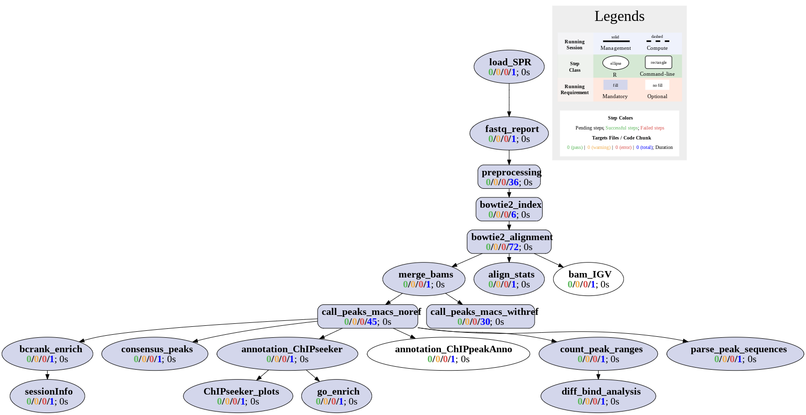
Toplogy graph of ChIP-Seq workflow.
Scientific and technical reports can be generated with the renderReport and
renderLogs functions, respectively. Scientific reports can also be generated
with the render function of the rmarkdown package. The latter option with
rmarkdown::render is often more flexible and preferred for most users, since
it provides the advantage that any modifications to the Rmd file are instantly
reflected in the HTML report, eliminating the necessity to update the sal
object. The technical reports are based on log information that systemPipeR
collects during workflow runs.
# Scientific report
sal <- renderReport(sal)
rmarkdown::render("systemPipeChIPseq.Rmd", clean = TRUE, output_format = "BiocStyle::html_document")

# Technical (log) report
sal <- renderLogs(sal)
The statusWF function returns a status summary for each step in a SAL workflow instance.
statusWF(sal)
Workflow steps
The data analysis steps of this workflow are defined by the following workflow code chunks.
They can be loaded into SAL interactively, by executing the code of each step in the
R console, or all at once with the importWF function used under the Quick start section.
R and CL workflow steps are declared in the code chunks of Rmd files with the
LineWise and SYSargsList functions, respectively, and then added to the SAL workflow
container with appendStep<-. Their syntax and usage is described
here.
Load packages
The first step loads the systemPipeR package.
cat(crayon::blue$bold("To use this workflow, following R packages are expected:\n"))
cat(c("'ggbio", "ChIPseeker", "GenomicFeatures", "GenomicRanges",
    "Biostrings", "seqLogo", "BCRANK", "readr'\n"), sep = "', '")
targetspath <- system.file("extdata", "targetsPE_chip.txt", package = "systemPipeR")
### pre-end
appendStep(sal) <- LineWise(code = {
    library(systemPipeR)
}, step_name = "load_SPR")
Read preprocessing
FASTQ quality report
The following seeFastq and seeFastqPlot functions generate and plot a series of useful
quality statistics for a set of FASTQ files, including per cycle quality box
plots, base proportions, base-level quality trends, relative k-mer
diversity, length, and occurrence distribution of reads, number of reads
above quality cutoffs and mean quality distribution. The results are
written to a png file named fastqReport.png.
This is the pre-trimming fastq report. Another post-trimming fastq report step is not included in the default. It is recommended to run this step first to decide whether the trimming is needed.
Please note that initial targets files are being used here. In this case,
it has been added to the first step using the updateColumn function, and
later, we used the getColumn function to extract a named vector.
appendStep(sal) <- LineWise(code = {
    targets <- read.delim(targetspath, comment.char = "#")
    updateColumn(sal, step = "load_SPR", position = "targetsWF") <- targets
    fq_files <- getColumn(sal, "load_SPR", "targetsWF", column = 1)
    fqlist <- seeFastq(fastq = fq_files, batchsize = 10000, klength = 8)
    png("./results/fastqReport.png", height = 1500, width = 330 *
        length(fqlist))
    seeFastqPlot(fqlist)
    dev.off()
}, step_name = "fastq_report", dependency = "load_SPR")
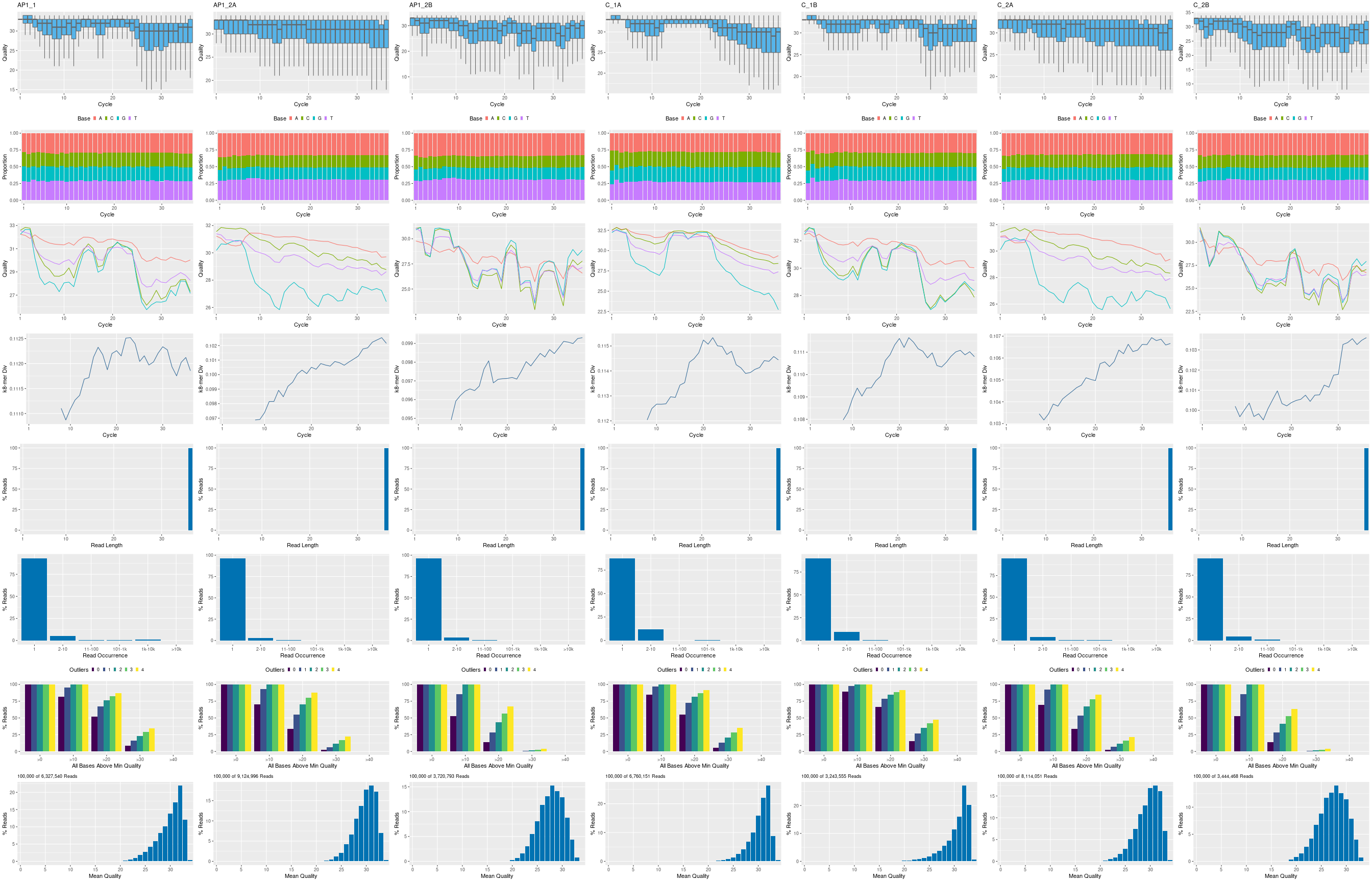
Figure 1: FASTQ quality report for 18 samples
Preprocessing with preprocessReads function
The function preprocessReads allows to apply predefined or custom
read preprocessing functions to all FASTQ files referenced in a
SYSargsList container, such as quality filtering or adapter trimming
routines. Internally, preprocessReads uses the FastqStreamer function from
the ShortRead package to stream through large FASTQ files in a
memory-efficient manner. The following example performs adapter trimming with
the trimLRPatterns function from the Biostrings package.
Here, we are appending this step to the SYSargsList object created previously.
All the parameters are defined on the preprocessReads-pe.yml file.
appendStep(sal) <- SYSargsList(step_name = "preprocessing", targets = targetspath,
    dir = TRUE, wf_file = "preprocessReads/preprocessReads-pe.cwl",
    input_file = "preprocessReads/preprocessReads-pe.yml", dir_path = system.file("extdata/cwl",
        package = "systemPipeR"), inputvars = c(FileName1 = "_FASTQ_PATH1_",
        FileName2 = "_FASTQ_PATH2_", SampleName = "_SampleName_"),
    dependency = c("fastq_report"))
After the preprocessing step, the outfiles files can be used to generate the new
targets files containing the paths to the trimmed FASTQ files. The new targets
information can be used for the next workflow step instance, e.g. running the
NGS alignments with the trimmed FASTQ files. The appendStep function is
automatically handling this connectivity between steps. Please check the next
step for more details.
The following example shows how one can design a custom read ‘preprocessReads’
function using utilities provided by the ShortRead package, and then run it
in batch mode with the ‘preprocessReads’ function. Here, it is possible to
replace the function used on the preprocessing step and modify the sal object.
Because it is a custom function, it is necessary to save the part in the R object,
and internally the preprocessReads.doc.R is loading the custom function.
If the R object is saved with a different name (here "param/customFCT.RData"),
please replace that accordingly in the preprocessReads.doc.R.
Please, note that this step is not added to the workflow, here just for demonstration.
First, we defined the custom function in the workflow:
appendStep(sal) <- LineWise(code = {
    filterFct <- function(fq, cutoff = 20, Nexceptions = 0) {
        qcount <- rowSums(as(quality(fq), "matrix") <= cutoff,
            na.rm = TRUE)
        # Retains reads where Phred scores are >= cutoff
        # with N exceptions
        fq[qcount <= Nexceptions]
    }
    save(list = ls(), file = "param/customFCT.RData")
}, step_name = "custom_preprocessing_function", dependency = "preprocessing")
After, we can edit the input parameter:
yamlinput(sal, "preprocessing")$Fct
yamlinput(sal, "preprocessing", "Fct") <- "'filterFct(fq, cutoff=20, Nexceptions=0)'"
yamlinput(sal, "preprocessing")$Fct  ## check the new function
cmdlist(sal, "preprocessing", targets = 1)  ## check if the command line was updated with success
Alignments
Read mapping with Bowtie2
The NGS reads of this project will be aligned with Bowtie2 against the
reference genome sequence (Langmead and Salzberg 2012). The parameter settings of the
Bowtie2 index are defined in the bowtie2-index.cwl and bowtie2-index.yml files.
Building the index:
appendStep(sal) <- SYSargsList(step_name = "bowtie2_index", dir = FALSE,
    targets = NULL, wf_file = "bowtie2/bowtie2-index.cwl", input_file = "bowtie2/bowtie2-index.yml",
    dir_path = system.file("extdata/cwl", package = "systemPipeR"),
    inputvars = NULL, dependency = c("preprocessing"))
The parameter settings of the aligner are defined in the workflow_bowtie2-pe.cwl
and workflow_bowtie2-pe.yml files. The following shows how to construct the
corresponding SYSargsList object.
In ChIP-Seq experiments it is usually more appropriate to eliminate reads mapping
to multiple locations. To achieve this, users want to remove the argument setting
-k 50 non-deterministic in the configuration files.
appendStep(sal) <- SYSargsList(step_name = "bowtie2_alignment",
    dir = TRUE, targets = targetspath, wf_file = "workflow-bowtie2/workflow_bowtie2-pe.cwl",
    input_file = "workflow-bowtie2/workflow_bowtie2-pe.yml",
    dir_path = system.file("extdata/cwl", package = "systemPipeR"),
    inputvars = c(FileName1 = "_FASTQ_PATH1_", FileName2 = "_FASTQ_PATH2_",
        SampleName = "_SampleName_"), dependency = c("bowtie2_index"))
To double-check the command line for each sample, please use the following:
cmdlist(sal, step = "bowtie2_alignment", targets = 1)
Read and alignment stats
The following provides an overview of the number of reads in each sample and how many of them aligned to the reference.
appendStep(sal) <- LineWise(code = {
    fqpaths <- getColumn(sal, step = "bowtie2_alignment", "targetsWF",
        column = "FileName1")
    bampaths <- getColumn(sal, step = "bowtie2_alignment", "outfiles",
        column = "samtools_sort_bam")
    read_statsDF <- alignStats(args = bampaths, fqpaths = fqpaths,
        pairEnd = TRUE)
    write.table(read_statsDF, "results/alignStats.xls", row.names = FALSE,
        quote = FALSE, sep = "\t")
}, step_name = "align_stats", dependency = "bowtie2_alignment")
Create symbolic links for viewing BAM files in IGV
The symLink2bam function creates symbolic links to view the BAM alignment files in a
genome browser such as IGV without moving these large files to a local
system. The corresponding URLs are written to a file with a path
specified under urlfile, here IGVurl.txt.
Please replace the directory and the user name.
appendStep(sal) <- LineWise(code = {
    bampaths <- getColumn(sal, step = "bowtie2_alignment", "outfiles",
        column = "samtools_sort_bam")
    symLink2bam(sysargs = bampaths, htmldir = c("~/.html/", "somedir/"),
        urlbase = "http://cluster.hpcc.ucr.edu/~tgirke/", urlfile = "./results/IGVurl.txt")
}, step_name = "bam_IGV", dependency = "bowtie2_alignment", run_step = "optional")
Utilities for coverage data
The following introduces several utilities useful for ChIP-Seq data. They are not part of the actual workflow. These utilities can be explored once the workflow is executed.
Rle object stores coverage information
bampaths <- getColumn(sal, step = "bowtie2_alignment", "outfiles",
    column = "samtools_sort_bam")
aligns <- readGAlignments(bampaths[1])
cov <- coverage(aligns)
cov
Resizing aligned reads
trim(resize(as(aligns, "GRanges"), width = 200))
Naive peak calling
islands <- slice(cov, lower = 15)
islands[[1]]
Plot coverage for defined region
library(ggbio)
myloc <- c("Chr1", 1, 1e+05)
ga <- readGAlignments(bampaths[1], use.names = TRUE, param = ScanBamParam(which = GRanges(myloc[1],
    IRanges(as.numeric(myloc[2]), as.numeric(myloc[3])))))
autoplot(ga, aes(color = strand, fill = strand), facets = strand ~
    seqnames, stat = "coverage")
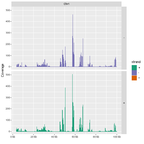
Figure 2: Plot coverage for chromosome 1 region.
Peak calling with MACS2
Merge BAM files of replicates prior to peak calling
Merging BAM files of technical and/or biological replicates can improve
the sensitivity of the peak calling by increasing the depth of read
coverage. The mergeBamByFactor function merges BAM files based on grouping information
specified by a factor, here the Factor column of the imported targets file.
It also returns an updated targets object containing the paths to the
merged BAM files as well as to any unmerged files without replicates.
The updated targets object can be used to update the SYSargsList object.
This step can be skipped if merging of BAM files is not desired.
appendStep(sal) <- LineWise(code = {
    bampaths <- getColumn(sal, step = "bowtie2_alignment", "outfiles",
        column = "samtools_sort_bam")
    merge_bams <- mergeBamByFactor(args = bampaths, targetsDF = targetsWF(sal)[["bowtie2_alignment"]],
        out_dir = file.path("results", "merge_bam"), overwrite = TRUE)
    updateColumn(sal, step = "merge_bams", position = "targetsWF") <- merge_bams
}, step_name = "merge_bams", dependency = "bowtie2_alignment")
Peak calling without input/reference sample
MACS2 can perform peak calling on ChIP-Seq data with and without input
samples (Zhang et al. 2008). The following performs peak calling without
input on all samples specified in the corresponding targets object. Note, due to
the small size of the sample data, MACS2 needs to be run here with the
nomodel setting. For real data sets, users want to remove this parameter
in the corresponding *.param file(s).
cat("Running preprocessing for call_peaks_macs_noref\n")
# Previous Linewise step is not run at workflow building
# time, but we need the output as input for this sysArgs
# step. So we use some preprocess code to predict the
# output paths to update the output targets of merge_bams,
# and then them into this next step during workflow
# building phase.
mergebam_out_dir = file.path("results", "merge_bam")  # make sure this is the same output directory used in merge_bams
targets_merge_bam <- targetsWF(sal)$bowtie2_alignment
targets_merge_bam <- targets_merge_bam[, -which(colnames(targets_merge_bam) %in%
    c("FileName1", "FileName2", "FileName"))]
targets_merge_bam <- targets_merge_bam[!duplicated(targets_merge_bam$Factor),
    ]
targets_merge_bam <- cbind(FileName = file.path(mergebam_out_dir,
    paste0(targets_merge_bam$Factor, "_merged.bam")), targets_merge_bam)
updateColumn(sal, step = "merge_bams", position = "targetsWF") <- targets_merge_bam
# write it out as backup, so you do not need to use
# preprocess code above again
writeTargets(sal, step = "merge_bams", file = "targets_merge_bams.txt",
    overwrite = TRUE)

### pre-end
appendStep(sal) <- SYSargsList(step_name = "call_peaks_macs_noref",
    targets = "targets_merge_bams.txt", wf_file = "MACS2/macs2-noinput.cwl",
    input_file = "MACS2/macs2-noinput.yml", dir_path = system.file("extdata/cwl",
        package = "systemPipeR"), inputvars = c(FileName = "_FASTQ_PATH1_",
        SampleName = "_SampleName_"), dependency = c("merge_bams"))
Peak calling with input/reference sample
To perform peak calling with input samples, they can be most
conveniently specified in the SampleReference column of the initial
targets file. The writeTargetsRef function uses this information to create a targets
file intermediate for running MACS2 with the corresponding input samples.
cat("Running preprocessing for call_peaks_macs_withref\n")
# To generate the reference targets file for the next step,
# use `writeTargetsRef`, this file needs to be present at
# workflow building time Use following preprocess code to
# do so:
writeTargetsRef(infile = "targets_merge_bams.txt", outfile = "targets_bam_ref.txt",
    silent = FALSE, overwrite = TRUE)

### pre-end
appendStep(sal) <- SYSargsList(step_name = "call_peaks_macs_withref",
    targets = "targets_bam_ref.txt", wf_file = "MACS2/macs2-input.cwl",
    input_file = "MACS2/macs2-input.yml", dir_path = system.file("extdata/cwl",
        package = "systemPipeR"), inputvars = c(FileName1 = "_FASTQ_PATH1_",
        FileName2 = "_FASTQ_PATH2_", SampleName = "_SampleName_"),
    dependency = c("merge_bams"))
The peak calling results from MACS2 are written for each sample to
separate files in the results/call_peaks_macs_withref directory. They are named after the corresponding files with extensions used by MACS2.
Identify consensus peaks
The following example shows how one can identify consensus peaks among two peak sets sharing either a minimum absolute overlap and/or minimum relative overlap using the subsetByOverlaps or olRanges functions, respectively. Note, the latter is a custom function imported below by sourcing it.
appendStep(sal) <- LineWise(code = {
    peaks_files <- getColumn(sal, step = "call_peaks_macs_noref",
        "outfiles", column = "peaks_xls")
    peak_M1A <- peaks_files["M1A"]
    peak_M1A <- as(read.delim(peak_M1A, comment = "#")[, 1:3],
        "GRanges")
    peak_A1A <- peaks_files["A1A"]
    peak_A1A <- as(read.delim(peak_A1A, comment = "#")[, 1:3],
        "GRanges")
    (myol1 <- subsetByOverlaps(peak_M1A, peak_A1A, minoverlap = 1))
    # Returns any overlap
    myol2 <- olRanges(query = peak_M1A, subject = peak_A1A, output = "gr")
    # Returns any overlap with OL length information
    myol2[values(myol2)["OLpercQ"][, 1] >= 50]
    # Returns only query peaks with a minimum overlap of
    # 50%
}, step_name = "consensus_peaks", dependency = "call_peaks_macs_noref")
Annotate peaks with genomic context
Annotation with ChIPseeker package
The following annotates the identified peaks with genomic context information
using the ChIPseeker package (Yu, Wang, and He 2015).
appendStep(sal) <- LineWise(code = {
    library(ChIPseeker)
    library(GenomicFeatures)
    peaks_files <- getColumn(sal, step = "call_peaks_macs_noref",
        "outfiles", column = "peaks_xls")
    txdb <- suppressWarnings(makeTxDbFromGFF(file = "data/tair10.gff",
        format = "gff", dataSource = "TAIR", organism = "Arabidopsis thaliana"))
    for (i in seq(along = peaks_files)) {
        peakAnno <- annotatePeak(peaks_files[i], TxDb = txdb,
            verbose = FALSE)
        df <- as.data.frame(peakAnno)
        outpaths <- paste0("./results/", names(peaks_files),
            "_ChIPseeker_annotated.xls")
        names(outpaths) <- names(peaks_files)
        write.table(df, outpaths[i], quote = FALSE, row.names = FALSE,
            sep = "\t")
    }
    updateColumn(sal, step = "annotation_ChIPseeker", position = "outfiles") <- data.frame(outpaths)
}, step_name = "annotation_ChIPseeker", dependency = "call_peaks_macs_noref")
The peak annotation results are written for each peak set to separate
files in the results/ directory.
Summary plots provided by the ChIPseeker package. Here applied only to one sample
for demonstration purposes.
appendStep(sal) <- LineWise(code = {
    peaks_files <- getColumn(sal, step = "call_peaks_macs_noref",
        "outfiles", column = "peaks_xls")
    peak <- readPeakFile(peaks_files[1])
    png("results/peakscoverage.png")
    covplot(peak, weightCol = "X.log10.pvalue.")
    dev.off()
    png("results/peaksHeatmap.png")
    peakHeatmap(peaks_files[1], TxDb = txdb, upstream = 1000,
        downstream = 1000, color = "red")
    dev.off()
    png("results/peaksProfile.png")
    plotAvgProf2(peaks_files[1], TxDb = txdb, upstream = 1000,
        downstream = 1000, xlab = "Genomic Region (5'->3')",
        ylab = "Read Count Frequency", conf = 0.05)
    dev.off()
}, step_name = "ChIPseeker_plots", dependency = "annotation_ChIPseeker")
Annotation with ChIPpeakAnno package
Same as in previous step but using the ChIPpeakAnno package (Zhu et al. 2010) for
annotating the peaks.
appendStep(sal) <- LineWise(code = {
    library(ChIPpeakAnno)
    library(GenomicFeatures)
    peaks_files <- getColumn(sal, step = "call_peaks_macs_noref",
        "outfiles", column = "peaks_xls")
    txdb <- suppressWarnings(makeTxDbFromGFF(file = "data/tair10.gff",
        format = "gff", dataSource = "TAIR", organism = "Arabidopsis thaliana"))
    ge <- genes(txdb, columns = c("tx_name", "gene_id", "tx_type"))
    for (i in seq(along = peaks_files)) {
        peaksGR <- as(read.delim(peaks_files[i], comment = "#"),
            "GRanges")
        annotatedPeak <- annotatePeakInBatch(peaksGR, AnnotationData = genes(txdb))
        df <- data.frame(as.data.frame(annotatedPeak), as.data.frame(values(ge[values(annotatedPeak)$feature,
            ])))
        df$tx_name <- as.character(lapply(df$tx_name, function(x) paste(unlist(x),
            sep = "", collapse = ", ")))
        df$tx_type <- as.character(lapply(df$tx_type, function(x) paste(unlist(x),
            sep = "", collapse = ", ")))
        outpaths <- paste0("./results/", names(peaks_files),
            "_ChIPpeakAnno_annotated.xls")
        names(outpaths) <- names(peaks_files)
        write.table(df, outpaths[i], quote = FALSE, row.names = FALSE,
            sep = "\t")
    }
}, step_name = "annotation_ChIPpeakAnno", dependency = "call_peaks_macs_noref",
    run_step = "optional")
The peak annotation results are written for each peak set to separate
files in the results/ directory.
Count reads overlapping peaks
The countRangeset function is a convenience wrapper to perform read counting
iteratively over several range sets, here peak range sets. Internally,
the read counting is performed with the summarizeOverlaps function from the
GenomicAlignments package. The resulting count tables are directly saved to
files, one for each peak set.
appendStep(sal) <- LineWise(code = {
    library(GenomicRanges)
    bam_files <- getColumn(sal, step = "bowtie2_alignment", "outfiles",
        column = "samtools_sort_bam")
    args <- getColumn(sal, step = "call_peaks_macs_noref", "outfiles",
        column = "peaks_xls")
    outfiles <- paste0("./results/", names(args), "_countDF.xls")
    bfl <- BamFileList(bam_files, yieldSize = 50000, index = character())
    countDFnames <- countRangeset(bfl, args, outfiles, mode = "Union",
        ignore.strand = TRUE)
    updateColumn(sal, step = "count_peak_ranges", position = "outfiles") <- data.frame(countDFnames)
}, step_name = "count_peak_ranges", dependency = "call_peaks_macs_noref",
    )
Differential binding analysis
The runDiff function performs differential binding analysis in batch mode for
several count tables using edgeR or DESeq2 (Robinson, McCarthy, and Smyth 2010; Love, Huber, and Anders 2014).
Internally, it calls the functions run_edgeR and run_DESeq2. It also returns
the filtering results and plots from the downstream filterDEGs function using
the fold change and FDR cutoffs provided under the dbrfilter argument.
appendStep(sal) <- LineWise(code = {
    countDF_files <- getColumn(sal, step = "count_peak_ranges",
        "outfiles")
    outfiles <- paste0("./results/", names(countDF_files), "_peaks_edgeR.xls")
    names(outfiles) <- names(countDF_files)
    cmp <- readComp(file = stepsWF(sal)[["bowtie2_alignment"]],
        format = "matrix")
    dbrlist <- runDiff(args = countDF_files, outfiles = outfiles,
        diffFct = run_edgeR, targets = targetsWF(sal)[["bowtie2_alignment"]],
        cmp = cmp[[1]], independent = TRUE, dbrfilter = c(Fold = 2,
            FDR = 1))
}, step_name = "diff_bind_analysis", dependency = "count_peak_ranges",
    )
GO term enrichment analysis
The following performs GO term enrichment analysis for each annotated peak set.
appendStep(sal) <- LineWise(code = {
    annofiles <- getColumn(sal, step = "annotation_ChIPseeker",
        "outfiles")
    gene_ids <- sapply(annofiles, function(x) unique(as.character(read.delim(x)[,
        "geneId"])), simplify = FALSE)
    load("data/GO/catdb.RData")
    BatchResult <- GOCluster_Report(catdb = catdb, setlist = gene_ids,
        method = "all", id_type = "gene", CLSZ = 2, cutoff = 0.9,
        gocats = c("MF", "BP", "CC"), recordSpecGO = NULL)
    write.table(BatchResult, "results/GOBatchAll.xls", quote = FALSE,
        row.names = FALSE, sep = "\t")
}, step_name = "go_enrich", dependency = "annotation_ChIPseeker",
    )
Motif analysis
Parse DNA sequences of peak regions from genome
Enrichment analysis of known DNA binding motifs or de novo discovery
of novel motifs requires the DNA sequences of the identified peak
regions. To parse the corresponding sequences from the reference genome,
the getSeq function from the Biostrings package can be used. The
following example parses the sequences for each peak set and saves the
results to separate FASTA files, one for each peak set. In addition, the
sequences in the FASTA files are ranked (sorted) by increasing p-values
as expected by some motif discovery tools, such as BCRANK.
appendStep(sal) <- LineWise(code = {
    library(Biostrings)
    library(seqLogo)
    library(BCRANK)
    rangefiles <- getColumn(sal, step = "call_peaks_macs_noref",
        "outfiles")
    for (i in seq(along = rangefiles)) {
        df <- read.delim(rangefiles[i], comment = "#")
        peaks <- as(df, "GRanges")
        names(peaks) <- paste0(as.character(seqnames(peaks)),
            "_", start(peaks), "-", end(peaks))
        peaks <- peaks[order(values(peaks)$X.log10.pvalue., decreasing = TRUE)]
        pseq <- getSeq(FaFile("./data/tair10.fasta"), peaks)
        names(pseq) <- names(peaks)
        writeXStringSet(pseq, paste0(rangefiles[i], ".fasta"))
    }
}, step_name = "parse_peak_sequences", dependency = "call_peaks_macs_noref",
    )
Motif discovery with BCRANK
The Bioconductor package BCRANK is one of the many tools available for
de novo discovery of DNA binding motifs in peak regions of ChIP-Seq
experiments. The given example applies this method on the first peak
sample set and plots the sequence logo of the highest ranking motif.
appendStep(sal) <- LineWise(code = {
    library(Biostrings)
    library(seqLogo)
    library(BCRANK)
    rangefiles <- getColumn(sal, step = "call_peaks_macs_noref",
        "outfiles")
    set.seed(0)
    BCRANKout <- bcrank(paste0(rangefiles[1], ".fasta"), restarts = 25,
        use.P1 = TRUE, use.P2 = TRUE)
    toptable(BCRANKout)
    topMotif <- toptable(BCRANKout, 1)
    weightMatrix <- pwm(topMotif, normalize = FALSE)
    weightMatrixNormalized <- pwm(topMotif, normalize = TRUE)
    png("results/seqlogo.png")
    seqLogo(weightMatrixNormalized)
    dev.off()
}, step_name = "bcrank_enrich", dependency = "call_peaks_macs_noref",
    )

Figure 3: One of the motifs identified by BCRANK
Version Information
appendStep(sal) <- LineWise(code = {
    sessionInfo()
}, step_name = "sessionInfo", dependency = "bcrank_enrich")
Running workflow
Interactive job submissions in a single machine
For running the workflow, runWF function will execute all the steps store in
the workflow container. The execution will be on a single machine without
submitting to a queuing system of a computer cluster.
sal <- runWF(sal)
Parallelization on clusters
Alternatively, the computation can be greatly accelerated by processing many files in parallel using several compute nodes of a cluster, where a scheduling/queuing system is used for load balancing.
The resources list object provides the number of independent parallel cluster
processes defined under the Njobs element in the list. The following example
will run 18 processes in parallel using each 4 CPU cores.
If the resources available on a cluster allow running all 18 processes at the
same time, then the shown sample submission will utilize in a total of 72 CPU cores.
Note, runWF can be used with most queueing systems as it is based on utilities
from the batchtools package, which supports the use of template files (*.tmpl)
for defining the run parameters of different schedulers. To run the following
code, one needs to have both a conffile (see .batchtools.conf.R samples here)
and a template file (see *.tmpl samples here)
for the queueing available on a system. The following example uses the sample
conffile and template files for the Slurm scheduler provided by this package.
The resources can be appended when the step is generated, or it is possible to
add these resources later, as the following example using the addResources
function:
# wall time in mins, memory in MB
resources <- list(conffile = ".batchtools.conf.R", template = "batchtools.slurm.tmpl",
    Njobs = 18, walltime = 120, ntasks = 1, ncpus = 4, memory = 1024,
    partition = "short")
sal <- addResources(sal, c("bowtie2_alignment"), resources = resources)
sal <- runWF(sal)
Visualize workflow
systemPipeR workflows instances can be visualized with the plotWF function.
plotWF(sal, rstudio = TRUE)
Checking workflow status
To check the summary of the workflow, we can use:
sal
statusWF(sal)
Accessing logs report
systemPipeR compiles all the workflow execution logs in one central location,
making it easier to check any standard output (stdout) or standard error
(stderr) for any command-line tools used on the workflow or the R code stdout.
sal <- renderLogs(sal)
If you are running on a single machine, use following code as an example to check if some tools used in this workflow are in your environment PATH. No warning message should be shown if all tools are installed.
Tools used
To check command-line tools used in this workflow, use listCmdTools, and use listCmdModules
to check if you have a modular system.
The following code will print out tools required in your custom SPR project in the report. In case you are running the workflow for the first time and do not have a project yet, or you just want to browser this workflow, following code displays the tools required by default.
if (file.exists(file.path(".SPRproject", "SYSargsList.yml"))) {
    local({
        sal <- systemPipeR::SPRproject(resume = TRUE)
        systemPipeR::listCmdTools(sal)
        systemPipeR::listCmdModules(sal)
    })
} else {
    cat(crayon::blue$bold("Tools and modules required by this workflow are:\n"))
    cat(c("BLAST 2.14.0+"), sep = "\n")
}
## Tools and modules required by this workflow are:
## BLAST 2.14.0+
Session Info
This is the session information for rendering this report. To access the session information
of workflow running, check HTML report of renderLogs.
sessionInfo()
## R version 4.4.3 (2025-02-28)
## Platform: x86_64-pc-linux-gnu
## Running under: Debian GNU/Linux 11 (bullseye)
##
## Matrix products: default
## BLAS:   /usr/lib/x86_64-linux-gnu/blas/libblas.so.3.9.0
## LAPACK: /usr/lib/x86_64-linux-gnu/lapack/liblapack.so.3.9.0
##
## locale:
##  [1] LC_CTYPE=en_US.UTF-8       LC_NUMERIC=C
##  [3] LC_TIME=en_US.UTF-8        LC_COLLATE=en_US.UTF-8
##  [5] LC_MONETARY=en_US.UTF-8    LC_MESSAGES=en_US.UTF-8
##  [7] LC_PAPER=en_US.UTF-8       LC_NAME=C
##  [9] LC_ADDRESS=C               LC_TELEPHONE=C
## [11] LC_MEASUREMENT=en_US.UTF-8 LC_IDENTIFICATION=C
##
## time zone: America/Los_Angeles
## tzcode source: system (glibc)
##
## attached base packages:
## [1] stats4    stats     graphics  grDevices utils
## [6] datasets  methods   base
##
## other attached packages:
##  [1] DT_0.33                     systemPipeRdata_2.10.0
##  [3] systemPipeR_2.12.0          ShortRead_1.64.0
##  [5] GenomicAlignments_1.42.0    SummarizedExperiment_1.36.0
##  [7] Biobase_2.66.0              MatrixGenerics_1.18.0
##  [9] matrixStats_1.4.1           BiocParallel_1.40.0
## [11] Rsamtools_2.22.0            Biostrings_2.74.0
## [13] XVector_0.46.0              GenomicRanges_1.58.0
## [15] GenomeInfoDb_1.42.1         IRanges_2.40.1
## [17] S4Vectors_0.44.0            BiocGenerics_0.52.0
## [19] BiocStyle_2.34.0
##
## loaded via a namespace (and not attached):
##  [1] gtable_0.3.6            xfun_0.49
##  [3] bslib_0.8.0             hwriter_1.3.2.1
##  [5] ggplot2_3.5.1           remotes_2.5.0
##  [7] htmlwidgets_1.6.4       latticeExtra_0.6-30
##  [9] lattice_0.22-6          generics_0.1.3
## [11] vctrs_0.6.5             tools_4.4.3
## [13] bitops_1.0-9            parallel_4.4.3
## [15] fansi_1.0.6             tibble_3.2.1
## [17] pkgconfig_2.0.3         Matrix_1.7-2
## [19] RColorBrewer_1.1-3      lifecycle_1.0.4
## [21] GenomeInfoDbData_1.2.13 stringr_1.5.1
## [23] compiler_4.4.3          deldir_2.0-4
## [25] munsell_0.5.1           codetools_0.2-20
## [27] htmltools_0.5.8.1       sass_0.4.9
## [29] yaml_2.3.10             pillar_1.9.0
## [31] crayon_1.5.3            jquerylib_0.1.4
## [33] DelayedArray_0.32.0     cachem_1.1.0
## [35] abind_1.4-8             tidyselect_1.2.1
## [37] digest_0.6.37           stringi_1.8.4
## [39] dplyr_1.1.4             bookdown_0.41
## [41] fastmap_1.2.0           grid_4.4.3
## [43] colorspace_2.1-1        cli_3.6.3
## [45] SparseArray_1.6.0       magrittr_2.0.3
## [47] S4Arrays_1.6.0          utf8_1.2.4
## [49] UCSC.utils_1.2.0        scales_1.3.0
## [51] rmarkdown_2.29          pwalign_1.2.0
## [53] httr_1.4.7              jpeg_0.1-10
## [55] interp_1.1-6            blogdown_1.19
## [57] png_0.1-8               evaluate_1.0.1
## [59] knitr_1.49              rlang_1.1.4
## [61] Rcpp_1.0.13-1           glue_1.8.0
## [63] formatR_1.14            BiocManager_1.30.25
## [65] jsonlite_1.8.9          R6_2.5.1
## [67] zlibbioc_1.52.0
Funding
This project was supported by funds from the National Institutes of Health (NIH) and the National Science Foundation (NSF).
References
H Backman, Tyler W, and Thomas Girke. 2016. “systemPipeR: NGS workflow and report generation environment.” BMC Bioinformatics 17 (1): 388. https://doi.org/10.1186/s12859-016-1241-0.
Howard, Brian E, Qiwen Hu, Ahmet Can Babaoglu, Manan Chandra, Monica Borghi, Xiaoping Tan, Luyan He, et al. 2013. “High-Throughput RNA Sequencing of Pseudomonas-Infected Arabidopsis Reveals Hidden Transcriptome Complexity and Novel Splice Variants.” PLoS One 8 (10): e74183. https://doi.org/10.1371/journal.pone.0074183.
Langmead, Ben, and Steven L Salzberg. 2012. “Fast Gapped-Read Alignment with Bowtie 2.” Nat. Methods 9 (4): 357–59. https://doi.org/10.1038/nmeth.1923.
Love, Michael, Wolfgang Huber, and Simon Anders. 2014. “Moderated Estimation of Fold Change and Dispersion for RNA-seq Data with DESeq2.” Genome Biol. 15 (12): 550. https://doi.org/10.1186/s13059-014-0550-8.
Robinson, M D, D J McCarthy, and G K Smyth. 2010. “EdgeR: A Bioconductor Package for Differential Expression Analysis of Digital Gene Expression Data.” Bioinformatics 26 (1): 139–40. https://doi.org/10.1093/bioinformatics/btp616.
Yu, Guangchuang, Li-Gen Wang, and Qing-Yu He. 2015. “ChIPseeker: An R/Bioconductor Package for ChIP Peak Annotation, Comparison and Visualization.” Bioinformatics 31 (14): 2382–3. https://doi.org/10.1093/bioinformatics/btv145.
Zhang, Y, T Liu, C A Meyer, J Eeckhoute, D S Johnson, B E Bernstein, C Nussbaum, et al. 2008. “Model-Based Analysis of ChIP-Seq (MACS).” Genome Biol. 9 (9). https://doi.org/10.1186/gb-2008-9-9-r137.
Zhu, Lihua J, Claude Gazin, Nathan D Lawson, Hervé Pagès, Simon M Lin, David S Lapointe, and Michael R Green. 2010. “ChIPpeakAnno: A Bioconductor Package to Annotate ChIP-seq and ChIP-chip Data.” BMC Bioinformatics 11: 237. https://doi.org/10.1186/1471-2105-11-237.