R Markdown Tutorial
10 minute read
R Markdown Overview
R Markdown combines markdown (an easy to write plain text format) with embedded
R code chunks. When compiling R Markdown documents, the code components can be
evaluated so that both the code and its output can be included in the final
document. This makes analysis reports highly reproducible by allowing to automatically
regenerate them when the underlying R code or data changes. R Markdown
documents (.Rmd files) can be rendered to various formats including HTML and
PDF. The R code in an .Rmd document is processed by knitr, while the
resulting .md file is rendered by pandoc to the final output formats
(e.g. HTML or PDF). Historically, R Markdown is an extension of the older
Sweave/Latex environment. Rendering of mathematical expressions and reference
management is also supported by R Markdown using embedded Latex syntax and
Bibtex, respectively. A new and related publishing environemt is Quarto (not covered here).
Quick Start
Install R Markdown
To work with this tutorial, the rmarkdown package needs to be installed on a system.
install.packages("rmarkdown")
Initialize a new R Markdown (Rmd) script
To minimize typing, it can be helful to start with an R Markdown template and
then modify it as needed. Note the file name of an R Markdown scirpt needs to
have the extension .Rmd. Template files for the following examples are available
here:
- R Markdown sample script:
sample.Rmd - Bibtex file for handling citations and reference section:
bibtex.bib
Users want to download these files, open the sample.Rmd file with their preferred R IDE
(e.g. RStudio, vim or emacs), initilize an R session and then direct their R session to
the location of these two files.
Metadata section
The metadata section (YAML header) in an R Markdown script defines how it will be processed and
rendered. The metadata section also includes both title, author, and date information as well as
options for customizing the output format. For instance, PDF and HTML output can be defined
with pdf_document and html_document, respectively. The BiocStyle:: prefix will use the
formatting style of the BiocStyle
package from Bioconductor.
 ---
title: "My First R Markdown Document"
author: "Author: First Last"
date: "Last update: 08 June, 2025"
output:
  BiocStyle::html_document:
    toc: true
    toc_depth: 3
    fig_caption: yes

fontsize: 14pt
bibliography: bibtex.bib
 ---
Render Rmd script
An R Markdown script can be evaluated and rendered with the following render command or by pressing the knit button in RStudio.
The output_format argument defines the format of the output (e.g. html_document or pdf_document). The setting output_format="all" will generate
all supported output formats. Alternatively, one can specify several output formats in the metadata section.
rmarkdown::render("sample.Rmd", clean=TRUE, output_format="BiocStyle::html_document")
The following shows two options how to run the rendering from the command-line. To render to PDF format, use the argument setting: output_format="pdf_document".
$ Rscript -e "rmarkdown::render('sample.Rmd', output_format='BiocStyle::html_document', clean=TRUE)"
Alternatively, one can use a Makefile to evaluate and render an R Markdown
script. A sample Makefile for rendering the above sample.Rmd can be
downloaded here.
To apply it to a custom Rmd file, one needs open the Makefile in a text
editor and change the value assigned to MAIN (line 13) to the base name of
the corresponding .Rmd file (e.g. assign systemPipeRNAseq if the file
name is systemPipeRNAseq.Rmd). To execute the Makefile, run the following
command from the command-line.
$ make -B
R code chunks
R Code Chunks can be embedded in an R Markdown script by using three backticks at the beginning of a new line along with arguments enclosed in curly braces controlling the behavior of the code. The following lines contain the plain R code. A code chunk is terminated by a new line starting with three backticks. The following shows an example of such a code chunk. Note the backslashes are not part of it. They have been added to print the code chunk syntax in this document.
	```\{r code_chunk_name, eval=FALSE\}
	x <- 1:10
	```
The following lists the most important arguments to control the behavior of R code chunks:
r: specifies language for code chunk, here Rchode_chunk_name: name of code chunk; this name needs to be unique within an Rmdeval: if assignedTRUEthe code will be evaluatedwarning: if assignedFALSEwarnings will not be shownmessage: if assignedFALSEmessages will not be showncache: if assignedTRUEresults will be cached to reuse in future rendering instancesfig.height: allows to specify height of figures in inchesfig.width: allows to specify width of figures in inches
For more details on code chunk options see here.
If document rendering of code chunk sections becomes time consuming due to long computations, one can enable caching to improve performance.
The corresponding cache options of the knitr package describes how caching works and the cache examples here provide additional details.
Learning Markdown
The basic syntax of Markdown and derivatives like kramdown is extremely easy to learn. Rather than providing another introduction on this topic, here are some useful sites for learning Markdown:
- R Markdown Online Book
- Markdown Intro on GitHub
- Markdown Cheet Sheet
- Markdown Basics from RStudio
- R Markdown Cheat Sheet
- kramdown Syntax
Tables
There are several ways to render tables. First, they can be printed within the R code chunks. Second,
much nicer formatted tables can be generated with the functions kable, kableExtra, pander or xtable. The following
example uses kable from the knitr package.
With knitr::kable
library(knitr)
kable(iris[1:12,])
| Sepal.Length | Sepal.Width | Petal.Length | Petal.Width | Species |
|---|---|---|---|---|
| 5.1 | 3.5 | 1.4 | 0.2 | setosa |
| 4.9 | 3.0 | 1.4 | 0.2 | setosa |
| 4.7 | 3.2 | 1.3 | 0.2 | setosa |
| 4.6 | 3.1 | 1.5 | 0.2 | setosa |
| 5.0 | 3.6 | 1.4 | 0.2 | setosa |
| 5.4 | 3.9 | 1.7 | 0.4 | setosa |
| 4.6 | 3.4 | 1.4 | 0.3 | setosa |
| 5.0 | 3.4 | 1.5 | 0.2 | setosa |
| 4.4 | 2.9 | 1.4 | 0.2 | setosa |
| 4.9 | 3.1 | 1.5 | 0.1 | setosa |
| 5.4 | 3.7 | 1.5 | 0.2 | setosa |
| 4.8 | 3.4 | 1.6 | 0.2 | setosa |
A much more elegant and powerful solution is to create fully interactive tables with the DT package.
This JavaScirpt based environment provides a wrapper to the DataTables library using jQuery. The resulting tables can be sorted, queried and resized by the
user. Note, R Markdown source files containing JavaScript components can only be rendered into HTML and not PDF.
With DT::datatable
library(DT)
datatable(iris)
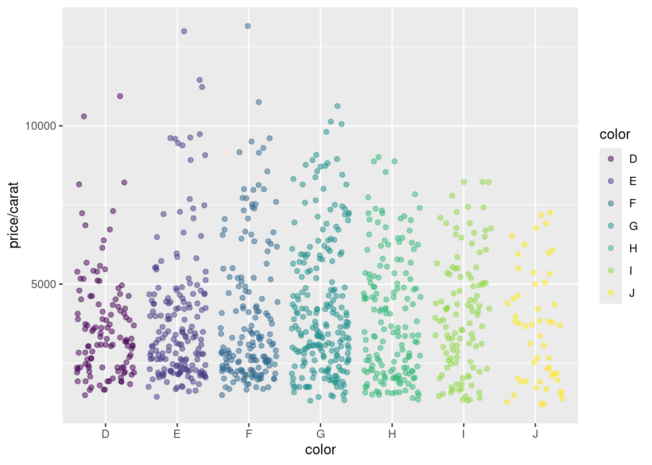
Figures
Plots generated by the R code chunks in an R Markdown document can be automatically
inserted in the output file. The size of the figure can be controlled with the fig.height
and fig.width arguments.
library(ggplot2)
dsmall <- diamonds[sample(nrow(diamonds), 1000), ]
ggplot(dsmall, aes(color, price/carat)) + geom_jitter(alpha = I(1 / 2), aes(color=color))
Sometimes it can be useful to explicitly write an image to a file and then insert that
image into the final document by referencing its file name in the R Markdown source. For
instance, this can be useful for time consuming analyses. The following code will generate a
file named myplot.png. To insert the file in the final document, one can use standard
Markdown or HTML syntax, e.g.: <img src="myplot.png"/>.
png("myplot.png")
ggplot(dsmall, aes(color, price/carat)) + geom_jitter(alpha = I(1 / 2), aes(color=color))
dev.off()
## png
##   2

Custom functions
Custom functions can be kept in a separate R file (here custom_Fct.R) and then imported
with the source() command. In the following example, the custom_Fct.R file is located on GitHub.
source("https://raw.githubusercontent.com/tgirke/GEN242/main/content/en/tutorials/rmarkdown/custom_Fct.R")
Now the imported function (here myMAcomp) can be used.
myMA <- matrix(rnorm(100000), 10000, 10, dimnames=list(1:10000, paste("C", 1:10, sep="")))
resultDF <- myMAcomp(myMA=myMA, group=c(1,1,1,2,2,2,3,3,4,4), myfct=mean)
kable(resultDF[1:12,])
| C1_C2_C3 | C4_C5_C6 | C7_C8 | C9_C10 |
|---|---|---|---|
| 0.7822402 | 1.0855980 | -0.9855508 | -0.4183372 |
| -0.3477805 | 0.3508050 | 1.0365380 | 1.7736885 |
| 0.7198847 | 0.7264769 | 0.6953388 | 0.1562494 |
| -0.5400569 | -0.4686734 | 0.0366285 | -0.2591983 |
| -0.5173485 | 0.3565092 | -0.9244651 | 0.5881874 |
| 0.2466624 | -0.0421876 | -0.5582115 | -0.4154806 |
| -0.8029628 | -0.1590556 | 0.5684271 | -0.8062521 |
| 0.8440542 | -0.1031945 | 0.0356007 | -0.1089801 |
| 0.4848108 | 0.2441012 | 1.1716362 | 0.9396260 |
| -0.7510482 | 0.4705989 | 0.4838571 | -0.1798379 |
| 0.5765647 | -0.1467300 | -0.3005206 | -0.0749069 |
| 0.1267778 | -0.1564793 | -0.2159484 | -0.3942560 |
Inline R code
To evaluate R code inline, one can enclose an R expression with a single back-tick
followed by r and then the actual expression. For instance, the back-ticked version
of ‘r 1 + 1’ evaluates to 2 and ‘r pi’ evaluates to 3.1415927.
Mathematical equations
To render mathematical equations, one can use standard Latex syntax. When expressions are
enclosed with single $ signs then they will be shown inline, while
enclosing them with double $$ signs will show them in display mode. For instance, the following
Latex syntax d(X,Y) = \sqrt[]{ \sum_{i=1}^{n}{(x_{i}-y_{i})^2} } renders in display mode as follows:
$$d(X,Y) = \sqrt[]{ \sum_{i=1}^{n}{(x_{i}-y_{i})^2} }$$
To learn LaTeX syntax for mathematical equations, one can consult various online manuals, such as this Wikibooks tutorial, or use an online equation rendering and checking tool, such as this one.
Citations and bibliographies
Citations and bibliographies can be autogenerated in R Markdown in a similar
way as in Latex/Bibtex. Reference collections should be stored in a separate
file in Bibtex or other supported formats. To cite a publication in an R Markdown
script, one uses the syntax [@<id1>] where <id1> needs to be replaced with a
reference identifier present in the Bibtex database listed in the metadata section
of the R Markdown script (e.g. bibtex.bib). For instance, to cite Lawrence et al.
(2013), one uses its reference identifier (e.g. Lawrence2013-kt) as <id1> (Lawrence et al. 2013).
This will place the citation inline in the text and add the corresponding
reference to a reference list at the end of the output document. For the latter a
special section called References needs to be specified at the end of the R Markdown script.
To fine control the formatting of citations and reference lists, users want to consult this
R Markdown page.
Also, for general reference management and obtaining references in Bibtex format Paperpile
can be very helpful.
Viewing R Markdown report on HPCC cluster
R Markdown reports located on UCR’s HPCC Cluster can be viewed locally in a web browser (without moving
the source HTML) by creating a symbolic link from a user’s .html directory. This way any updates to
the report will show up immediately without creating another copy of the HTML file. For instance, if user
ttest has generated an R Markdown report under ~/bigdata/today/rmarkdown/sample.html, then the
symbolic link can be created as follows:
cd ~/.html
ln -s ~/bigdata/today/rmarkdown/sample.html sample.html
After this one can view the report in a web browser using this URL https://cluster.hpcc.ucr.edu/~ttest/rmarkdown/sample.html. If necessary access to the URL can be restricted with a password following the instructions here. Very important: to set up accounts for html viewing, users have to apply the configuration settings for their accounts that are outlined on the HPCC website here.
Viewing R Markdown report on GitHub
To host and view static HTML files on GitHub, follow the instructions here. Note, this works only with public GitHub repos.
Session Info
sessionInfo()
## R version 4.4.3 (2025-02-28)
## Platform: x86_64-pc-linux-gnu
## Running under: Debian GNU/Linux 11 (bullseye)
##
## Matrix products: default
## BLAS:   /usr/lib/x86_64-linux-gnu/blas/libblas.so.3.9.0
## LAPACK: /usr/lib/x86_64-linux-gnu/lapack/liblapack.so.3.9.0
##
## locale:
##  [1] LC_CTYPE=en_US.UTF-8       LC_NUMERIC=C
##  [3] LC_TIME=en_US.UTF-8        LC_COLLATE=en_US.UTF-8
##  [5] LC_MONETARY=en_US.UTF-8    LC_MESSAGES=en_US.UTF-8
##  [7] LC_PAPER=en_US.UTF-8       LC_NAME=C
##  [9] LC_ADDRESS=C               LC_TELEPHONE=C
## [11] LC_MEASUREMENT=en_US.UTF-8 LC_IDENTIFICATION=C
##
## time zone: America/Los_Angeles
## tzcode source: system (glibc)
##
## attached base packages:
## [1] stats     graphics  grDevices utils     datasets  methods   base
##
## other attached packages:
## [1] ggplot2_3.5.1 DT_0.33       knitr_1.49
##
## loaded via a namespace (and not attached):
##  [1] gtable_0.3.6      jsonlite_1.8.9    dplyr_1.1.4       compiler_4.4.3
##  [5] tidyselect_1.2.1  jquerylib_0.1.4   scales_1.3.0      yaml_2.3.10
##  [9] fastmap_1.2.0     R6_2.5.1          labeling_0.4.3    generics_0.1.3
## [13] htmlwidgets_1.6.4 tibble_3.2.1      bookdown_0.41     munsell_0.5.1
## [17] bslib_0.8.0       pillar_1.9.0      rlang_1.1.4       utf8_1.2.4
## [21] cachem_1.1.0      xfun_0.49         sass_0.4.9        viridisLite_0.4.2
## [25] cli_3.6.3         withr_3.0.2       magrittr_2.0.3    crosstalk_1.2.1
## [29] digest_0.6.37     grid_4.4.3        lifecycle_1.0.4   vctrs_0.6.5
## [33] evaluate_1.0.1    glue_1.8.0        farver_2.1.2      blogdown_1.19
## [37] fansi_1.0.6       colorspace_2.1-1  rmarkdown_2.29    tools_4.4.3
## [41] pkgconfig_2.0.3   htmltools_0.5.8.1
References
Lawrence, Michael, Wolfgang Huber, Hervé Pagès, Patrick Aboyoun, Marc Carlson, Robert Gentleman, Martin T Morgan, and Vincent J Carey. 2013. “Software for Computing and Annotating Genomic Ranges.” PLoS Comput. Biol. 9 (8): e1003118. https://doi.org/10.1371/journal.pcbi.1003118.