RNA-Seq Workflow Template
29 minute read
Introduction
Overview
This workflow template is for analyzing RNA-Seq data. It is provided by
systemPipeRdata,
a companion package to systemPipeR (H Backman and Girke 2016).
Similar to other systemPipeR workflow templates, a single command generates
the necessary working environment. This includes the expected directory
structure for executing systemPipeR workflows and parameter files for running
command-line (CL) software utilized in specific analysis steps. For learning
and testing purposes, a small sample (toy) data set is also included (mainly
FASTQ and reference genome files). This enables users to seamlessly run the
numerous analysis steps of this workflow from start to finish without the
requirement of providing custom data. After testing the workflow, users have
the flexibility to employ the template as is with their own data or modify it
to suit their specific needs. For more comprehensive information on designing
and executing workflows, users want to refer to the main vignettes of
systemPipeR
and
systemPipeRdata.
The Rmd file (systemPipeRNAseq.Rmd) associated with this vignette serves a dual purpose. It acts
both as a template for executing the workflow and as a template for generating
a reproducible scientific analysis report. Thus, users want to customize the text
(and/or code) of this vignette to describe their experimental design and
analysis results. This typically involves deleting the instructions how to work
with this workflow, and customizing the text describing experimental designs,
other metadata and analysis results.
Experimental design
Typically, the user wants to describe here the sources and versions of the
reference genome sequence along with the corresponding annotations. The standard
directory structure of systemPipeR (see here),
expects the input data in a subdirectory named data
and all results will be written to a separate results directory. The Rmd source file
for executing the workflow and rendering its report (here systemPipeRNAseq.Rmd) is
expected to be located in the parent directory.
The test (toy) data set used by this template (SRP010938) contains 18 paired-end (PE) read sets from Arabidposis thaliana (Howard et al. 2013). To minimize processing time during testing, each FASTQ file has been reduced to 90,000-100,000 randomly sampled PE reads that map to the first 100,000 nucleotides of each chromosome of the A. thaliana genome. The corresponding reference genome sequence (FASTA) and its GFF annotation files have been reduced to the same genome regions. This way the entire test sample data set is less than 200MB in storage space. A PE read set has been chosen here for flexibility, because it can be used for testing both types of analysis routines requiring either SE (single end) reads or PE reads.
To use their own RNA-Seq and reference genome data, users want to move or link the
data to the designated data directory and execute the workflow from the parent directory
using their customized Rmd file. Beginning with this template, users should delete the provided test
data and move or link their custom data to the designated locations.
Alternatively, users can create an environment skeleton (named new here) or
build one from scratch. To perform an RNA-Seq analysis with new FASTQ files
from the same reference genome, users only need to provide the FASTQ files and
an experimental design file called ‘targets’ file that outlines the experimental
design. The structure and utility of targets files is described in systemPipeR's
main vignette here.
Workflow steps
The default analysis steps included in this RNA-Seq workflow template are listed below. Users can modify the existing steps, add new ones or remove steps as needed.
Default analysis steps
- Read preprocessing
- Quality filtering (trimming)
- FASTQ quality report
- Alignments:
HISAT2(or any other RNA-Seq aligner) - Alignment stats
- Read counting
- Sample-wise correlation analysis
- Analysis of differentially expressed genes (DEGs)
- GO term enrichment analysis
- Gene-wise clustering
Setup of workflow environment
NOTE: this section describes how to set up the proper
environment (directory structure) for running systemPipeR workflows in the GEN242
class. This routine applies to all workflows. After mastering this task the workflow
run instructions can be deleted since they are not expected
to be included in a final HTML/PDF report of a workflow.
-
If a remote system or cluster is used, then users need to log in to the remote system first. The following applies to an HPC cluster (e.g. HPCC cluster).
A terminal application or RStudion Server via onDemand needs to be used to log in to a user’s cluster account. Next, one can open an interactive session on a computer node with
srun. More details about argument settings forsrunare available in this HPCC manual or the HPCC section of this website here. Next, load the R version required for running the workflow withmodule load. Sometimes it may be necessary to first unload an active software version before loading another version, e.g.module unload R.
From command-line
srun --x11 --partition=gen242 --account=gen242 --mem=20gb --cpus-per-task 8 --ntasks 1 --time 20:00:00 --pty bash -l
module unload R; module load R/4.4.2
- Load a workflow template with the
genWorkenvirfunction. This can be done from the command-line or from within R. However, only one of the two options needs to be used.
The environment for this RNA-Seq workflow is auto-generated below with the
genWorkenvir function (selected under workflow="rnaseq"). It is fully populated
with a small test data set, including FASTQ files, reference genome and annotation data. The name of the
resulting workflow directory can be specified under the mydirname argument.
The default NULL uses the name of the chosen workflow. An error is issued if
a directory of the same name and path exists already. After this, the user’s R
session needs to be directed into the resulting rnaseq directory (here with
setwd).
From command-line
Rscript -e "systemPipeRdata::genWorkenvir(workflow='rnaseq')"
cd rnaseq
From R
library(systemPipeRdata)
genWorkenvir(workflow = "rnaseq", mydirname = "rnaseq")
setwd("rnaseq")
- If the user wishes to use another
Rmdfile than the template instance provided by thegenWorkenvirfunction, then it can be copied or downloaded into the root directory of the workflow environment (e.g. withcp,download.fileorwget). For the first introduction to RNA-Seq analysis in GEN242, we will use theRmdfile obtained bygenWorkenvir. Note, theRmdsource file of this tutorial page is linked on the top.
# From command-line
wget <*.Rmd> -O <*.Rmd>
# From R
download.file("<*.Rmd>", "*.Rmd>")
- Now one can open from the root directory of the workflow the corresponding R Markdown script (e.g. systemPipeChIPseq.Rmd) using an R IDE, such as nvim-r, ESS or RStudio. Subsequently, the workflow can be run as outlined below.
Import custom functions
Custom functions for the challenge projects can be imported with the source command from a local R script (here challengeProject_Fct.R). Skip this step if such a script is not available. Alternatively, these functions can be loaded from a custom R package.
source("challengeProject_Fct.R")
Input data: targets file
The targets file defines the input files (e.g. FASTQ or BAM) and sample
comparisons used in a data analysis workflow. It can also store any number of
additional descriptive information for each sample. The following shows the first
four lines of the targets file used in this workflow template.
targetspath <- system.file("extdata", "targetsPE.txt", package = "systemPipeR")
targets <- read.delim(targetspath, comment.char = "#")
targets[1:4, -c(5, 6)]
##                     FileName1                   FileName2
## 1 ./data/SRR446027_1.fastq.gz ./data/SRR446027_2.fastq.gz
## 2 ./data/SRR446028_1.fastq.gz ./data/SRR446028_2.fastq.gz
## 3 ./data/SRR446029_1.fastq.gz ./data/SRR446029_2.fastq.gz
## 4 ./data/SRR446030_1.fastq.gz ./data/SRR446030_2.fastq.gz
##   SampleName Factor        Date
## 1        M1A     M1 23-Mar-2012
## 2        M1B     M1 23-Mar-2012
## 3        A1A     A1 23-Mar-2012
## 4        A1B     A1 23-Mar-2012
To work with custom data, users need to generate a targets file containing
the paths to their own FASTQ files. Here is a detailed description of the structure and
utility of targets files.
Quick start
After a workflow environment has been created with the above genWorkenvir
function call and the corresponding R session directed into the resulting directory (here rnaseq),
the SPRproject function is used to initialize a new workflow project instance. The latter
creates an empty SAL workflow container (below sal) and at the same time a
linked project log directory (default name .SPRproject) that acts as a
flat-file database of a workflow. Additional details about this process and
the SAL workflow control class are provided in systemPipeR's main vignette
here
and here.
Next, the importWF function imports all the workflow steps outlined in the
source Rmd file of this vignette (here systemPipeRNAseq.Rmd) into the SAL workflow container.
An overview of the workflow steps and their status information can be returned
at any stage of the loading or run process by typing sal.
library(systemPipeR)
sal <- SPRproject()  # Intializes new workflow.
# sal <- SPRproject(resume=TRUE, load.envir=TRUE) #
# Restarts workflow.  sal <- SPRproject(overwrite=TRUE) #
# Resets workflow.
sal <- importWF(sal, file_path = "systemPipeRNAseq.Rmd", verbose = FALSE)
sal
After loading the workflow into sal, it can be executed from start to finish
(or partially) with the runWF command. Running the workflow will only be
possible if all dependent CL software is installed on a user’s system. Their
names and availability on a system can be listed with listCmdTools(sal, check_path=TRUE). For more information about the runWF command, refer to the
help file and the corresponding section in the main vignette
here.
Running workflows in parallel mode on computer clusters is a straightforward
process in systemPipeR. Users can simply append the resource parameters (such
as the number of CPUs) for a cluster run to the sal object after importing
the workflow steps with importWF using the addResources function. More
information about parallelization can be found in the corresponding section at
the end of this vignette here and in the main vignette
here.
sal <- runWF(sal)
Workflows can be visualized as topology graphs using the plotWF function.
plotWF(sal)
Toplogy graph of RNA-Seq workflow.
Scientific and technical reports can be generated with the renderReport and
renderLogs functions, respectively. Scientific reports can also be generated
with the render function of the rmarkdown package. The latter option with
rmarkdown::render is often more flexible and preferred for most users, since it
provides the advantage that any modifications to the
Rmd file are instantly reflected in the HTML report, eliminating the necessity
to update the sal object. The technical reports are based on log information that
systemPipeR collects during workflow runs.
# Scientific report
sal <- renderReport(sal)
rmarkdown::render("systemPipeRNAseq.Rmd", clean = TRUE, output_format = "BiocStyle::html_document")

# Technical (log) report
sal <- renderLogs(sal)
The statusWF function returns a status summary for each step in a SAL workflow instance.
statusWF(sal)
Workflow steps
The data analysis steps of this workflow are defined by the following workflow code chunks.
They can be loaded into SAL interactively, by executing the code of each step in the
R console, or all at once with the importWF function used under the Quick start section.
R and CL workflow steps are declared in the code chunks of Rmd files with the
LineWise and SYSargsList functions, respectively, and then added to the SAL workflow
container with appendStep<-. Their syntax and usage is described
here.
Load packages
The first step loads the systemPipeR package.
cat(crayon::blue$bold("To use this workflow, the following R packages are required:\n"))
cat(c("'GenomicFeatures", "BiocParallel", "DESeq2", "ape", "edgeR",
    "biomaRt", "pheatmap", "ggplot2'\n"), sep = "', '")
### pre-end
appendStep(sal) <- LineWise(code = {
    library(systemPipeR)
}, step_name = "load_SPR")
Read preprocessing
With preprocessReads
The preprocessReads function allows applying predefined or custom read
preprocessing functions to all FASTQ files referenced in a SAL container, such
as quality filtering or adapter trimming routines. Internally, preprocessReads
uses the FastqStreamer function from the ShortRead package to stream through
large FASTQ files in a memory-efficient manner. The following example uses
preprocessReads to perform adapter trimming with the trimLRPatterns function
from the Biostrings package. In this instance, preprocessReads is invoked
through a CL interface built on docopt, that is executed from R with CWL. The
parameters for running preprocessReads are specified in the corresponding
cwl/yml files. It is important to point out that creating and using CL
interfaces for defining R-based workflow steps is not essential in systemPipeR
since LineWise
offers similar capabilities while requiring less specialized
knowledge from users.
appendStep(sal) <- SYSargsList(step_name = "preprocessing", targets = "targetsPE.txt",
    dir = TRUE, wf_file = "preprocessReads/preprocessReads-pe.cwl",
    input_file = "preprocessReads/preprocessReads-pe.yml", dir_path = system.file("extdata/cwl",
        package = "systemPipeR"), inputvars = c(FileName1 = "_FASTQ_PATH1_",
        FileName2 = "_FASTQ_PATH2_", SampleName = "_SampleName_"),
    dependency = c("load_SPR"))
The paths to the output files generated by the preprocessing step (here trimmed FASTQ files)
are recorded in a new targets file that can be used for the next workflow step,
e.g. running the NGS alignments with the trimmed FASTQ files.
The following example demonstrates how to design a custom preprocessReads
function, as well as how to replace parameters in the sal object. To apply the
modifications to the workflow, it needs to be saved to a file, here param/customFCT.RData
which will be loaded during the workflow run by the preprocessReads.doc.R script.
Please note, this step is included here solely for demonstration purposes, and thus not
part of the workflow run. This is achieved by dropping spr=TRUE in the header line of the
code chunk.
appendStep(sal) <- LineWise(code = {
    filterFct <- function(fq, cutoff = 20, Nexceptions = 0) {
        qcount <- rowSums(as(quality(fq), "matrix") <= cutoff,
            na.rm = TRUE)
        # Retains reads where Phred scores are >= cutoff
        # with N exceptions
        fq[qcount <= Nexceptions]
    }
    save(list = ls(), file = "param/customFCT.RData")
}, step_name = "custom_preprocessing_function", dependency = "preprocessing")
After defining this step, it can be inspected and modified as follows.
yamlinput(sal, "preprocessing")$Fct
yamlinput(sal, "preprocessing", "Fct") <- "'filterFct(fq, cutoff=20, Nexceptions=0)'"
yamlinput(sal, "preprocessing")$Fct  ## check the new function
cmdlist(sal, "preprocessing", targets = 1)  ## check if the command line was updated with success
With Trimmomatic
For demonstration purposes, this workflow uses the Trimmomatic software as an example of an external CL read trimming tool (Bolger, Lohse, and Usadel 2014). Trimmomatic offers a range of practical trimming utilities specifically designed for single- and paired-end Illumina reads.
It is important to note that while the Trimmomatic trimming step is included in
this workflow, it’s not mandatory. Users can opt to use read trimming results
generated by the previous preprocessReads step if preferred.
appendStep(sal) <- SYSargsList(step_name = "trimming", targets = "targetsPE.txt",
    wf_file = "trimmomatic/trimmomatic-pe.cwl", input_file = "trimmomatic/trimmomatic-pe.yml",
    dir_path = system.file("extdata/cwl", package = "systemPipeR"),
    inputvars = c(FileName1 = "_FASTQ_PATH1_", FileName2 = "_FASTQ_PATH2_",
        SampleName = "_SampleName_"), dependency = "load_SPR",
    run_step = "optional")
FASTQ quality report
The following seeFastq and seeFastqPlot functions generate and plot a
series of useful quality statistics for a set of FASTQ files, including per
cycle quality box plots, base proportions, base-level quality trends, relative
k-mer diversity, length, and occurrence distribution of reads, number of reads
above quality cutoffs and mean quality distribution. The results can be
exported to different graphics formats, such as a PNG file, here named
fastqReport.png. Detailed information about the usage and visual components
in the quality plots can be found in the corresponding help file (see
?seeFastq or ?seeFastqPlot).
appendStep(sal) <- LineWise(code = {
    fastq <- getColumn(sal, step = "preprocessing", "targetsWF",
        column = 1)
    fqlist <- seeFastq(fastq = fastq, batchsize = 10000, klength = 8)
    png("./results/fastqReport.png", height = 1500, width = 330 *
        length(fqlist))
    seeFastqPlot(fqlist)
    dev.off()
}, step_name = "fastq_report", dependency = "preprocessing")
Figure 1: FASTQ quality report for 18 samples
Short read alignments
Read mapping with HISAT2
To use the HISAT2 short read aligner developed by Kim, Langmead, and Salzberg
(2015), it is necessary to index the reference genome. HISAT2 relies on the
Burrows-Wheeler index for this process.
appendStep(sal) <- SYSargsList(step_name = "hisat2_index", dir = FALSE,
    targets = NULL, wf_file = "hisat2/hisat2-index.cwl", input_file = "hisat2/hisat2-index.yml",
    dir_path = "param/cwl", dependency = "load_SPR")
HISAT2 mapping
The parameter settings of the aligner are defined in the cwl/yml files used
in the following code chunk. The following shows how to construct the alignment
step and append it to the SAL workflow container. Please note that the input
(FASTQ) files used in this step are the output files generated by the
preprocessing step (see above: step_name = "preprocessing").
appendStep(sal) <- SYSargsList(step_name = "hisat2_mapping",
    dir = TRUE, targets = "preprocessing", wf_file = "workflow-hisat2/workflow_hisat2-pe.cwl",
    input_file = "workflow-hisat2/workflow_hisat2-pe.yml", dir_path = "param/cwl",
    inputvars = c(preprocessReads_1 = "_FASTQ_PATH1_", preprocessReads_2 = "_FASTQ_PATH2_",
        SampleName = "_SampleName_"), rm_targets_col = c("FileName1",
        "FileName2"), dependency = c("preprocessing", "hisat2_index"))
The cmdlist functions allows to inspect the exact CL call used for each input file (sample), here
for HISAT2 alignments. Note, this step also includes the conversion of the alignment files to sorted
and indexed bam files using functionalities of the SAMtools CL suite.
cmdlist(sal, step = "hisat2_mapping", targets = 1)
$hisat2_mapping
$hisat2_mapping$M1A
$hisat2_mapping$M1A$hisat2
[1] "hisat2 -S ./results/M1A.sam  -x ./data/tair10.fasta  -k 1  --min-intronlen
30  --max-intronlen 3000  -1 ./results/M1A_1.fastq_trim.gz -2 ./results/M1A_2.fa
stq_trim.gz --threads 4"

$hisat2_mapping$M1A$`samtools-view`
[1] "samtools view -bS -o ./results/M1A.bam  ./results/M1A.sam "

$hisat2_mapping$M1A$`samtools-sort`
[1] "samtools sort -o ./results/M1A.sorted.bam  ./results/M1A.bam  -@ 4"

$hisat2_mapping$M1A$`samtools-index`
[1] "samtools index -b results/M1A.sorted.bam  results/M1A.sorted.bam.bai  ./res
ults/M1A.sorted.bam "
Alignment stats
The following computes an alignment summary file (here alignStats.xls), which
comprises the count of reads in each FASTQ file and the number of reads that
align with the reference, presented in both total and percentage values.
appendStep(sal) <- LineWise(code = {
    fqpaths <- getColumn(sal, step = "preprocessing", "targetsWF",
        column = "FileName1")
    bampaths <- getColumn(sal, step = "hisat2_mapping", "outfiles",
        column = "samtools_sort_bam")
    read_statsDF <- alignStats(args = bampaths, fqpaths = fqpaths,
        pairEnd = TRUE)
    write.table(read_statsDF, "results/alignStats.xls", row.names = FALSE,
        quote = FALSE, sep = "\t")
}, step_name = "align_stats", dependency = "hisat2_mapping")
The resulting alignStats.xls file can be included in the report as shown below (here restricted to the
first four rows).
read.table("results/alignStats.xls", header = TRUE)[1:4, ]
##   FileName Nreads2x Nalign Perc_Aligned Nalign_Primary
## 1      M1A   115994 109977     94.81266         109977
## 2      M1B   134480 112464     83.62879         112464
## 3      A1A   127976 122427     95.66403         122427
## 4      A1B   122486 101369     82.75966         101369
##   Perc_Aligned_Primary
## 1             94.81266
## 2             83.62879
## 3             95.66403
## 4             82.75966
Viewing BAM files in IGV
The symLink2bam function creates symbolic links to view the BAM alignment files in a
genome browser such as IGV without moving these large files to a local
system. The corresponding URLs are written to a file with a path
specified under urlfile, here IGVurl.txt.
Please replace the directory and the user name.
The symLink2bam function creates symbolic links to view the BAM alignment files
in a genome browser such as IGV without moving these large files to a local
system. The corresponding URLs are written to a file with a path specified
under urlfile, here IGVurl.txt. To make the following code work, users need to
change the directory name (here <somedir>), and the url base and user names (here
<base_url> and <username>) to the corresponding names on their system.
appendStep(sal) <- LineWise(code = {
    bampaths <- getColumn(sal, step = "hisat2_mapping", "outfiles",
        column = "samtools_sort_bam")
    symLink2bam(sysargs = bampaths, htmldir = c("~/.html/", "<somedir>/"),
        urlbase = "<base_url>/~<username>/", urlfile = "./results/IGVurl.txt")
}, step_name = "bam_IGV", dependency = "hisat2_mapping", run_step = "optional")
Read quantification
Reads overlapping with annotation ranges of interest are counted for
each sample using the summarizeOverlaps function (Lawrence et al. 2013).
Most often the read counting is preformed for exonic gene regions. This can be
done in a strand-specific or non-strand-specific manner, while accounting for overlaps
among adjacent genes or ignoring them. Subsequently, the expression
count values can be normalized with different methods.
Gene annotation database
For efficient handling of annotation ranges obtained from GFF or GTF files,
they are organized within a TxDb object. Subsequently, the object is written
to a SQLite database file. It is important to note that this process only needs to
be performed once for a specific version of an annotation file.
appendStep(sal) <- LineWise(code = {
    library(GenomicFeatures)
    txdb <- suppressWarnings(makeTxDbFromGFF(file = "data/tair10.gff",
        format = "gff", dataSource = "TAIR", organism = "Arabidopsis thaliana"))
    saveDb(txdb, file = "./data/tair10.sqlite")
}, step_name = "create_db", dependency = "hisat2_mapping")
Read counting with summarizeOverlaps
The provided example employs non-strand-specific read counting while
disregarding overlaps between different genes. As normalization the example uses
reads per kilobase per million mapped reads (RPKM). The raw read count table
(countDFeByg.xls) and the corresponding RPKM table (rpkmDFeByg.xls) are written
to distinct files in the project’s results directory. Parallelization across
multiple CPU cores is achieved with the BiocParallel package. When supplying a
BamFileList as illustrated below, the summarizeOverlaps method defaults to
employing bplapply and the register interface from BiocParallel. The
MulticoreParam will utilize the number of cores returned by
parallel::detectCores if the number of workers is left unspecified. For
further information, refer to the help documentation by typing
help("summarizeOverlaps").
appendStep(sal) <- LineWise(code = {
    library(GenomicFeatures)
    library(BiocParallel)
    txdb <- loadDb("./data/tair10.sqlite")
    outpaths <- getColumn(sal, step = "hisat2_mapping", "outfiles",
        column = "samtools_sort_bam")
    eByg <- exonsBy(txdb, by = c("gene"))
    bfl <- BamFileList(outpaths, yieldSize = 50000, index = character())
    multicoreParam <- MulticoreParam(workers = 4)
    register(multicoreParam)
    registered()
    counteByg <- bplapply(bfl, function(x) summarizeOverlaps(eByg,
        x, mode = "Union", ignore.strand = TRUE, inter.feature = FALSE,
        singleEnd = FALSE, BPPARAM = multicoreParam))
    countDFeByg <- sapply(seq(along = counteByg), function(x) assays(counteByg[[x]])$counts)
    rownames(countDFeByg) <- names(rowRanges(counteByg[[1]]))
    colnames(countDFeByg) <- names(bfl)
    rpkmDFeByg <- apply(countDFeByg, 2, function(x) returnRPKM(counts = x,
        ranges = eByg))
    write.table(countDFeByg, "results/countDFeByg.xls", col.names = NA,
        quote = FALSE, sep = "\t")
    write.table(rpkmDFeByg, "results/rpkmDFeByg.xls", col.names = NA,
        quote = FALSE, sep = "\t")
    ## Creating a SummarizedExperiment object
    colData <- data.frame(row.names = SampleName(sal, "hisat2_mapping"),
        condition = getColumn(sal, "hisat2_mapping", position = "targetsWF",
            column = "Factor"))
    colData$condition <- factor(colData$condition)
    countDF_se <- SummarizedExperiment::SummarizedExperiment(assays = countDFeByg,
        colData = colData)
    ## Add results as SummarizedExperiment to the workflow
    ## object
    SE(sal, "read_counting") <- countDF_se
}, step_name = "read_counting", dependency = "create_db")
Importantly, when conducting statistical differential expression or abundance analysis using
methods like edgeR or DESeq2, the raw count values are the expected
input. RPKM values should be reserved for specialized applications, such as
manually inspecting expression levels across different genes or features.
Shows first 10 rows of countDFeByg.xls table.
countDF <- read.delim("results/countDFeByg.xls", row.names = 1,
    check.names = FALSE)[1:200, ]
DT::datatable(countDF, options = list(scrollX = TRUE, autoWidth = TRUE))
Sample-wise clustering
The sample-wise Spearman correlation coefficients are calculated from the rlog
transformed expression values (countDF_se) generated using the DESeq2 package.
These values are then converted into a distance matrix, which is subsequently
used for hierarchical clustering with the hclust function. The resulting
dendrogram is then saved as a PNG file named sample_tree.png.
appendStep(sal) <- LineWise(code = {
    library(DESeq2, quietly = TRUE)
    library(ape, warn.conflicts = FALSE)
    ## Extracting SummarizedExperiment object
    se <- SE(sal, "read_counting")
    dds <- DESeqDataSet(se, design = ~condition)
    d <- cor(assay(rlog(dds)), method = "spearman")
    hc <- hclust(dist(1 - d))
    png("results/sample_tree.png")
    plot.phylo(as.phylo(hc), type = "p", edge.col = "blue", edge.width = 2,
        show.node.label = TRUE, no.margin = TRUE)
    dev.off()
}, step_name = "sample_tree", dependency = "read_counting")

Figure 2: Correlation dendrogram of samples
Analysis of DEGs
The analysis of differentially expressed genes (DEGs) is performed with
the glm method of the edgeR package (Robinson, McCarthy, and Smyth 2010). The sample
comparisons used by this analysis are defined in the header lines of the
targets.txt file starting with <CMP>.
Run edgeR
appendStep(sal) <- LineWise(code = {
    library(edgeR)
    countDF <- read.delim("results/countDFeByg.xls", row.names = 1,
        check.names = FALSE)
    cmp <- readComp(stepsWF(sal)[["hisat2_mapping"]], format = "matrix",
        delim = "-")
    edgeDF <- run_edgeR(countDF = countDF, targets = targetsWF(sal)[["hisat2_mapping"]],
        cmp = cmp[[1]], independent = FALSE, mdsplot = "")
    write.table(edgeDF, "./results/edgeRglm_allcomp.xls", quote = FALSE,
        sep = "\t", col.names = NA)
}, step_name = "run_edger", dependency = "read_counting")
Note, to call DEGs with DESeq2 instead of edgeR, users can simply replace in the above code
‘run_edgeR’ with ‘run_DESeq2’.
Add gene descriptions
This step is optional. It appends functional descriptions obtained from BioMart to the DEG table.
appendStep(sal) <- LineWise(code = {
    library("biomaRt")
    m <- useMart("plants_mart", dataset = "athaliana_eg_gene",
        host = "https://plants.ensembl.org")
    desc <- getBM(attributes = c("tair_locus", "description"),
        mart = m)
    desc <- desc[!duplicated(desc[, 1]), ]
    descv <- as.character(desc[, 2])
    names(descv) <- as.character(desc[, 1])
    edgeDF <- data.frame(edgeDF, Desc = descv[rownames(edgeDF)],
        check.names = FALSE)
    write.table(edgeDF, "./results/edgeRglm_allcomp.xls", quote = FALSE,
        sep = "\t", col.names = NA)
}, step_name = "custom_annot", dependency = "run_edger")
Plot DEG results
Filter and plot DEG results for up and down regulated genes. The
definition of up and down is given in the corresponding help
file. To open it, type ?filterDEGs in the R console.
Note, due to the small number of genes in the toy dataset, the FDR cutoff in this example is set to an unreasonably large value. With real data sets this cutoff should be set to a much smaller value (often 1%, 5% or 10%).
appendStep(sal) <- LineWise(code = {
    edgeDF <- read.delim("results/edgeRglm_allcomp.xls", row.names = 1,
        check.names = FALSE)
    png("results/DEGcounts.png")
    DEG_list <- filterDEGs(degDF = edgeDF, filter = c(Fold = 2,
        FDR = 20))
    dev.off()
    write.table(DEG_list$Summary, "./results/DEGcounts.xls",
        quote = FALSE, sep = "\t", row.names = FALSE)
}, step_name = "filter_degs", dependency = "custom_annot")
Figure 3: Up and down regulated DEGs.
Venn diagrams of DEG sets
The overLapper function can compute Venn intersects for large numbers of sample
sets (up to 20 or more) and plots 2-5 way Venn diagrams. A useful
feature is the possibility to combine the counts from several Venn
comparisons with the same number of sample sets in a single Venn diagram
(here for 4 up and down DEG sets).
The overLapper function can compute Venn intersects for large numbers of sample sets (up to 20 or more) and plots 2-5 way Venn diagrams. A useful feature is the possibility to combine the counts from several Venn comparisons with the same number of sample sets in a single Venn diagram (here for 4 up and down DEG sets).
appendStep(sal) <- LineWise(code = {
    vennsetup <- overLapper(DEG_list$Up[6:9], type = "vennsets")
    vennsetdown <- overLapper(DEG_list$Down[6:9], type = "vennsets")
    png("results/vennplot.png")
    vennPlot(list(vennsetup, vennsetdown), mymain = "", mysub = "",
        colmode = 2, ccol = c("blue", "red"))
    dev.off()
}, step_name = "venn_diagram", dependency = "filter_degs")
Figure 4: Venn Diagram for 4 Up and Down DEG Sets
GO term enrichment analysis
Obtain gene-to-GO mappings
The following shows how to obtain gene-to-GO mappings from biomaRt (here for A.
thaliana) and how to organize them for the downstream GO term
enrichment analysis. Alternatively, the gene-to-GO mappings can be
obtained for many organisms from Bioconductor’s *.db genome annotation
packages or GO annotation files provided by various genome databases.
For each annotation this relatively slow preprocessing step needs to be
performed only once. Subsequently, the preprocessed data can be loaded
with the load function as shown in the next subsection.
appendStep(sal) <- LineWise(code = {
    library("biomaRt")
    # listMarts() # To choose BioMart database
    # listMarts(host='plants.ensembl.org')
    m <- useMart("plants_mart", host = "https://plants.ensembl.org")
    # listDatasets(m)
    m <- useMart("plants_mart", dataset = "athaliana_eg_gene",
        host = "https://plants.ensembl.org")
    # listAttributes(m) # Choose data types you want to
    # download
    go <- getBM(attributes = c("go_id", "tair_locus", "namespace_1003"),
        mart = m)
    go <- go[go[, 3] != "", ]
    go[, 3] <- as.character(go[, 3])
    go[go[, 3] == "molecular_function", 3] <- "F"
    go[go[, 3] == "biological_process", 3] <- "P"
    go[go[, 3] == "cellular_component", 3] <- "C"
    go[1:4, ]
    if (!dir.exists("./data/GO"))
        dir.create("./data/GO")
    write.table(go, "data/GO/GOannotationsBiomart_mod.txt", quote = FALSE,
        row.names = FALSE, col.names = FALSE, sep = "\t")
    catdb <- makeCATdb(myfile = "data/GO/GOannotationsBiomart_mod.txt",
        lib = NULL, org = "", colno = c(1, 2, 3), idconv = NULL)
    save(catdb, file = "data/GO/catdb.RData")
}, step_name = "get_go_annot", dependency = "filter_degs")
Batch GO term enrichment analysis
Apply the enrichment analysis to the DEG sets obtained the above differential
expression analysis. Note, in the following example the FDR filter is set
here to an unreasonably high value, simply because of the small size of the toy
data set used in this vignette. Batch enrichment analysis of many gene sets is
performed with the GOCluster_Report function. When method=all, it returns all GO terms passing
the p-value cutoff specified under the cutoff arguments. When method=slim,
it returns only the GO terms specified under the myslimv argument. The given
example shows how a GO slim vector for a specific organism can be obtained from
BioMart.
appendStep(sal) <- LineWise(code = {
    library("biomaRt")
    load("data/GO/catdb.RData")
    DEG_list <- filterDEGs(degDF = edgeDF, filter = c(Fold = 2,
        FDR = 50), plot = FALSE)
    up_down <- DEG_list$UporDown
    names(up_down) <- paste(names(up_down), "_up_down", sep = "")
    up <- DEG_list$Up
    names(up) <- paste(names(up), "_up", sep = "")
    down <- DEG_list$Down
    names(down) <- paste(names(down), "_down", sep = "")
    DEGlist <- c(up_down, up, down)
    DEGlist <- DEGlist[sapply(DEGlist, length) > 0]
    BatchResult <- GOCluster_Report(catdb = catdb, setlist = DEGlist,
        method = "all", id_type = "gene", CLSZ = 2, cutoff = 0.9,
        gocats = c("MF", "BP", "CC"), recordSpecGO = NULL)
    m <- useMart("plants_mart", dataset = "athaliana_eg_gene",
        host = "https://plants.ensembl.org")
    goslimvec <- as.character(getBM(attributes = c("goslim_goa_accession"),
        mart = m)[, 1])
    BatchResultslim <- GOCluster_Report(catdb = catdb, setlist = DEGlist,
        method = "slim", id_type = "gene", myslimv = goslimvec,
        CLSZ = 10, cutoff = 0.01, gocats = c("MF", "BP", "CC"),
        recordSpecGO = NULL)
    write.table(BatchResultslim, "results/GOBatchSlim.xls", row.names = FALSE,
        quote = FALSE, sep = "\t")
}, step_name = "go_enrich", dependency = "get_go_annot")
Plot batch GO term results
The data.frame generated by GOCluster can be plotted with the goBarplot function. Because of the
variable size of the sample sets, it may not always be desirable to show
the results from different DEG sets in the same bar plot. Plotting
single sample sets is achieved by subsetting the input data frame as
shown in the first line of the following example.
appendStep(sal) <- LineWise(code = {
    gos <- BatchResultslim[grep("M6-V6_up_down", BatchResultslim$CLID),
        ]
    gos <- BatchResultslim
    png("results/GOslimbarplotMF.png", height = 8, width = 10)
    goBarplot(gos, gocat = "MF")
    goBarplot(gos, gocat = "BP")
    goBarplot(gos, gocat = "CC")
    dev.off()
}, step_name = "go_plot", dependency = "go_enrich")
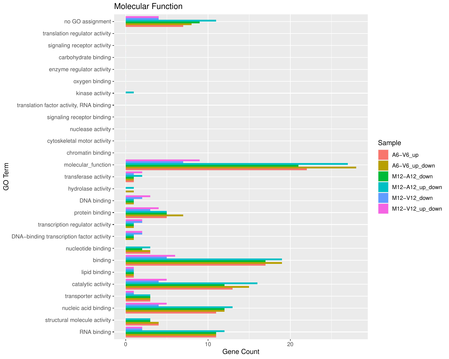
Figure 5: GO Slim Barplot for MF Ontology
Clustering and heat maps
The following example performs hierarchical clustering on the rlog
transformed expression matrix subsetted by the DEGs identified in the above
differential expression analysis. It uses a Pearson correlation-based distance
measure and complete linkage for cluster joining.
appendStep(sal) <- LineWise(code = {
    library(pheatmap)
    geneids <- unique(as.character(unlist(DEG_list[[1]])))
    y <- assay(rlog(dds))[geneids, ]
    png("results/heatmap1.png")
    pheatmap(y, scale = "row", clustering_distance_rows = "correlation",
        clustering_distance_cols = "correlation")
    dev.off()
}, step_name = "heatmap", dependency = "go_enrich")
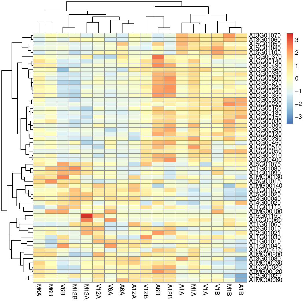
Figure 6: Heat Map with Hierarchical Clustering Dendrograms of DEGs
Workflow session information
appendStep(sal) <- LineWise(code = {
    sessionInfo()
}, step_name = "sessionInfo", dependency = "heatmap")
Additional details
Running workflows
The runWF function is the primary tool for executing workflows. It runs the
code of the workflow steps after loading them into a SAL workflow container.
The workflow steps can be loaded interactively one by one or in batch mode with
the importWF function. The batch mode is more convenient and is the intended
method for loading workflows. It is part of the standard routine for running
workflows introduced in the Quick start section.
Parallelization on clusters
The processing time of computationally expensive steps can be greatly accelerated by
processing many input files in parallel using several CPUs and/or computer nodes
of an HPC or cloud system, where a scheduling system is used for load balancing.
To simplify for users the configuration and execution of workflow steps in serial or parallel mode,
systemPipeR uses for both the same runWF function. Parallelization simply
requires appending of the parallelization parameters to the settings of the corresponding workflow
steps each requesting the computing resources specified by the user, such as
the number of CPU cores, RAM and run time. These resource settings are
stored in the corresponding workflow step of the SAL workflow container.
After adding the parallelization parameters, runWF will execute the chosen steps
in parallel mode as instructed.
The following example applies to an alignment step of an RNA-Seq workflow.
In the chosen alignment example, the parallelization
parameters are added to the alignment step (here hisat2_mapping) of SAL via
a resources list. The given parameter settings will run 18 processes (Njobs) in
parallel using for each 4 CPU cores (ncpus), thus utilizing a total of 72 CPU
cores. The runWF function can be used with most queueing systems as it is based on
utilities defined by the batchtools package, which supports the use of
template files (*.tmpl) for defining the run parameters of different
schedulers. In the given example below, a conffile (see
.batchtools.conf.R samples here) and
a template file (see *.tmpl samples
here) need to be present
on the highest level of a user’s workflow project. The following example uses the sample
conffile and template files for the Slurm scheduler that are both provided by this
package.
The resources list can be added to analysis steps when a workflow is loaded into SAL.
Alternatively, one can add the resource settings with the addResources function
to any step of a pre-populated SAL container afterwards. For workflow steps with the same resource
requirements, one can add them to several steps at once with a single call to addResources by
specifying multiple step names under the step argument.
resources <- list(conffile = ".batchtools.conf.R", template = "batchtools.slurm.tmpl",
    Njobs = 18, walltime = 120, ntasks = 1, ncpus = 4, memory = 1024,
    partition = "short")
sal <- addResources(sal, step = c("hisat2_mapping"), resources = resources)
sal <- runWF(sal)
The above example will submit via runWF(sal) the hisat2_mapping step
to a partition (queue) called short on an HPC cluster. Users need to adjust this and
other parameters, that are defined in the resources list, to their cluster environment .
CL tools used
The listCmdTools (and listCmdModules) return the CL tools that
are used by a workflow. To include a CL tool list in a workflow report,
one can use the following code. Additional details on this topic
can be found in the main vignette here.
if (file.exists(file.path(".SPRproject", "SYSargsList.yml"))) {
    local({
        sal <- systemPipeR::SPRproject(resume = TRUE)
        systemPipeR::listCmdTools(sal)
        systemPipeR::listCmdModules(sal)
    })
} else {
    cat(crayon::blue$bold("Tools and modules required by this workflow are:\n"))
    cat(c("gzip", "gunzip"), sep = "\n")
}
## Tools and modules required by this workflow are:
## gzip
## gunzip
Session info
This is the session information that will be included when rendering this report.
sessionInfo()
## R version 4.4.3 (2025-02-28)
## Platform: x86_64-pc-linux-gnu
## Running under: Debian GNU/Linux 11 (bullseye)
##
## Matrix products: default
## BLAS:   /usr/lib/x86_64-linux-gnu/blas/libblas.so.3.9.0
## LAPACK: /usr/lib/x86_64-linux-gnu/lapack/liblapack.so.3.9.0
##
## locale:
##  [1] LC_CTYPE=en_US.UTF-8       LC_NUMERIC=C
##  [3] LC_TIME=en_US.UTF-8        LC_COLLATE=en_US.UTF-8
##  [5] LC_MONETARY=en_US.UTF-8    LC_MESSAGES=en_US.UTF-8
##  [7] LC_PAPER=en_US.UTF-8       LC_NAME=C
##  [9] LC_ADDRESS=C               LC_TELEPHONE=C
## [11] LC_MEASUREMENT=en_US.UTF-8 LC_IDENTIFICATION=C
##
## time zone: America/Los_Angeles
## tzcode source: system (glibc)
##
## attached base packages:
## [1] stats4    stats     graphics  grDevices utils
## [6] datasets  methods   base
##
## other attached packages:
##  [1] DT_0.33                     batchtools_0.9.17
##  [3] ape_5.8-1                   ggplot2_3.5.1
##  [5] systemPipeR_2.12.0          ShortRead_1.64.0
##  [7] GenomicAlignments_1.42.0    SummarizedExperiment_1.36.0
##  [9] Biobase_2.66.0              MatrixGenerics_1.18.0
## [11] matrixStats_1.4.1           BiocParallel_1.40.0
## [13] Rsamtools_2.22.0            Biostrings_2.74.0
## [15] XVector_0.46.0              GenomicRanges_1.58.0
## [17] GenomeInfoDb_1.42.1         IRanges_2.40.1
## [19] S4Vectors_0.44.0            BiocGenerics_0.52.0
## [21] BiocStyle_2.34.0
##
## loaded via a namespace (and not attached):
##  [1] tidyselect_1.2.1        dplyr_1.1.4
##  [3] bitops_1.0-9            fastmap_1.2.0
##  [5] blogdown_1.19           digest_0.6.37
##  [7] base64url_1.4           lifecycle_1.0.4
##  [9] pwalign_1.2.0           magrittr_2.0.3
## [11] compiler_4.4.3          progress_1.2.3
## [13] rlang_1.1.4             sass_0.4.9
## [15] tools_4.4.3             utf8_1.2.4
## [17] yaml_2.3.10             data.table_1.16.4
## [19] knitr_1.49              prettyunits_1.2.0
## [21] brew_1.0-10             S4Arrays_1.6.0
## [23] htmlwidgets_1.6.4       interp_1.1-6
## [25] DelayedArray_0.32.0     RColorBrewer_1.1-3
## [27] abind_1.4-8             withr_3.0.2
## [29] hwriter_1.3.2.1         grid_4.4.3
## [31] fansi_1.0.6             latticeExtra_0.6-30
## [33] colorspace_2.1-1        scales_1.3.0
## [35] cli_3.6.3               rmarkdown_2.29
## [37] crayon_1.5.3            generics_0.1.3
## [39] httr_1.4.7              cachem_1.1.0
## [41] stringr_1.5.1           zlibbioc_1.52.0
## [43] parallel_4.4.3          formatR_1.14
## [45] BiocManager_1.30.25     vctrs_0.6.5
## [47] Matrix_1.7-2            jsonlite_1.8.9
## [49] bookdown_0.41           hms_1.1.3
## [51] jpeg_0.1-10             jquerylib_0.1.4
## [53] glue_1.8.0              codetools_0.2-20
## [55] stringi_1.8.4           gtable_0.3.6
## [57] deldir_2.0-4            UCSC.utils_1.2.0
## [59] munsell_0.5.1           tibble_3.2.1
## [61] pillar_1.9.0            rappdirs_0.3.3
## [63] htmltools_0.5.8.1       GenomeInfoDbData_1.2.13
## [65] R6_2.5.1                evaluate_1.0.1
## [67] lattice_0.22-6          png_0.1-8
## [69] backports_1.5.0         bslib_0.8.0
## [71] Rcpp_1.0.13-1           SparseArray_1.6.0
## [73] nlme_3.1-167            checkmate_2.3.2
## [75] xfun_0.49               pkgconfig_2.0.3
Funding
This project is funded by awards from the National Science Foundation (ABI-1661152], and the National Institute on Aging of the National Institutes of Health (U19AG023122).
References
Bolger, Anthony M, Marc Lohse, and Bjoern Usadel. 2014. “Trimmomatic: A Flexible Trimmer for Illumina Sequence Data.” Bioinformatics 30 (15): 2114–20.
H Backman, Tyler W, and Thomas Girke. 2016. “systemPipeR: NGS workflow and report generation environment.” BMC Bioinformatics 17 (1): 388. https://doi.org/10.1186/s12859-016-1241-0.
Howard, Brian E, Qiwen Hu, Ahmet Can Babaoglu, Manan Chandra, Monica Borghi, Xiaoping Tan, Luyan He, et al. 2013. “High-Throughput RNA Sequencing of Pseudomonas-Infected Arabidopsis Reveals Hidden Transcriptome Complexity and Novel Splice Variants.” PLoS One 8 (10): e74183. https://doi.org/10.1371/journal.pone.0074183.
Kim, Daehwan, Ben Langmead, and Steven L Salzberg. 2015. “HISAT: A Fast Spliced Aligner with Low Memory Requirements.” Nat. Methods 12 (4): 357–60.
Lawrence, Michael, Wolfgang Huber, Hervé Pagès, Patrick Aboyoun, Marc Carlson, Robert Gentleman, Martin T Morgan, and Vincent J Carey. 2013. “Software for Computing and Annotating Genomic Ranges.” PLoS Comput. Biol. 9 (8): e1003118. https://doi.org/10.1371/journal.pcbi.1003118.
Robinson, M D, D J McCarthy, and G K Smyth. 2010. “EdgeR: A Bioconductor Package for Differential Expression Analysis of Digital Gene Expression Data.” Bioinformatics 26 (1): 139–40. https://doi.org/10.1093/bioinformatics/btp616.