Programming in R

Author

Thomas Girke

Published

March 24, 2026

Overview

One of the main attractions of using the R (http://cran.at.r-project.org) environment is the ease with which users can write their own programs and custom functions. The R programming syntax is extremely easy to learn, even for users with no previous programming experience. Once the basic R programming control structures are understood, users can use the R language as a powerful environment to perform complex custom analyses of almost any type of data (Gentleman 2008).

Why Programming in R?

Powerful statistical environment and programming language
Facilitates reproducible research
Efficient data structures make programming very easy
Ease of implementing custom functions
Powerful graphics
Access to fast growing number of analysis packages
One of the most widely used languages in bioinformatics
Is standard for data mining and biostatistical analysis
Technical advantages: free, open-source, available for all OSs

R Basics

The previous Rbasics tutorial provides a general introduction to the usage of the R environment and its basic command syntax. More details can be found in the R & BioConductor manual here.

Code Editors for R

Several excellent code editors are available that provide functionalities like R syntax highlighting, auto code indenting and utilities to send code/functions to the R console.

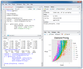
RStudio: GUI-based IDE for R
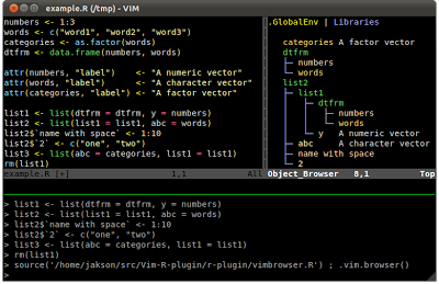
Vim-R-Tmux: R working environment based on vim and tmux
Emacs (ESS add-on package)
gedit and Rgedit
RKWard
Eclipse
Tinn-R
Notepad++ (NppToR)

R_Interfaces vim-r

Finding Help

Reference list on R programming (selection)

Advanced R, by Hadley Wickham
R Programming for Bioinformatics, by Robert Gentleman
S Programming, by W. N. Venables and B. D. Ripley
Programming with Data, by John M. Chambers
R Help & R Coding Conventions, Henrik Bengtsson, Lund University
Programming in R (Vincent Zoonekynd)
Peter’s R Programming Pages, University of Warwick
Rtips, Paul Johnsson, University of Kansas
R for Programmers, Norm Matloff, UC Davis
High-Performance R, Dirk Eddelbuettel tutorial presented at useR-2008
C/C++ level programming for R, Gopi Goswami

R Scripts

R programming involves the writing of R scripts, which are text files containing R code. The file name of an R script carries the extension .R (e.g. myscript.R). Typically, R scripts are composed of code sections, as well as comments (starting with #) explaining what the code does.

The structure and styling requirements of R scripts are not very strict. However, for maintainability and readability, it is highly recommended to follow widely adopted styling recommendations. For details on how to best and consistently format R scripts, this style guide is a good start. In addition, the formatR package is very helpful.

In addition to executing the code in R scripts interactively, e.g. line by line, one can execute R scripts as a whole with execution commands from the R console or the command-line using source or Rscript, respectively. The details on how to execute R scripts are explained in this section.

R Markdown (Rmd) and Quarto (qmd) scripts are an extension of R scripts that include in addition to R code, results and commentary text. Both can be rendered to a variety formats including HTML and PDF. They are explained in a separate tutorial here. R packages are often built for organizing more complex R code and providing usage instructions in the form of help files and vignettes (manuals). How to build R packages is explained in the R Package tutorial of this website.

The code in R scripts (or Rmd/qmd scripts) should be organized as much as possible in R functions that are called (used) somewhere in the script. Alternatively, functions can be organized in a secondary R script from where they are imported with the source command. This makes the code more concise, readable and reusable.

Control Structures

Important Operators

Comparison operators

== (equal)
!= (not equal)
> (greater than)
>= (greater than or equal)
< (less than)
<= (less than or equal)

Logical operators

& (and)
&& (and)
| (or)
|| (or)
! (not)

Note: & and && indicate logical AND, while | and || indicate logical OR. The shorter form performs element-wise comparisons of same-length vectors. The longer form evaluates left to right examining only the first element of each vector (can be of different lengths). Evaluation proceeds only until the result is determined. The longer form is preferred for programming control-flow, e.g. via if clauses.

Conditional Executions: `if` Statements

An if statement operates on length-one logical vectors.

Syntax

if (TRUE) { 
    statements_1 
} else { 
    statements_2 
}

In the else component, avoid inserting newlines between } else.

Example

if (1==0) { 
    print(1) 
} else { 
    print(2) 
}

[1] 2

Example 2

if (1==0) { 
    print(1) 
} else if (1==2) { 
    print(2) 
} else {
    print(3)
}

[1] 3

Conditional Executions: `ifelse` Statements

The ifelse statement operates on vectors.

Syntax

ifelse(test, true_value, false_value)

Example

x <- 1:10 
ifelse(x<5, sqrt(x), 0)

 [1] 1.000000 1.414214 1.732051 2.000000 0.000000 0.000000 0.000000 0.000000 0.000000 0.000000

Loops

`for` loop

for loops iterate over elements of a looping vector.

Syntax

for(variable in sequence) { 
    statements 
}

Example

mydf <- iris
myve <- NULL
for(i in seq(along=mydf[,1])) {
    myve <- c(myve, mean(as.numeric(mydf[i,1:3])))
}
myve[1:8]

[1] 3.333333 3.100000 3.066667 3.066667 3.333333 3.666667 3.133333 3.300000

Note: Inject into objecs is much faster than append approach with c, cbind, etc.

Example

myve <- numeric(length(mydf[,1]))
for(i in seq(along=myve)) {
    myve[i] <- mean(as.numeric(mydf[i,1:3]))
}
myve[1:8]

[1] 3.333333 3.100000 3.066667 3.066667 3.333333 3.666667 3.133333 3.300000

Conditional Stop of Loops

The stop function can be used to break out of a loop (or a function) when a condition becomes TRUE. In addition, an error message will be printed.

Example

x <- 1:10
z <- NULL
for(i in seq(along=x)) { 
    if (x[i] < 5) { 
        z <- c(z, x[i]-1)  
        print(z)
    } else { 
        stop("values need to be < 5") 
    }
}

`while` loop

Iterates as long as a condition is true.

Syntax

while(condition) {
    statements
}

Example

z <- 0
while(z<5) { 
    z <- z + 2
    print(z)  
}

[1] 2
[1] 4
[1] 6

The `apply` Function Family

`apply`

Syntax

apply(X, MARGIN, FUN, ARGs)

Arguments

X: array, matrix or data.frame
MARGIN: 1 for rows, 2 for columns
FUN: one or more functions
ARGs: possible arguments for functions

Example

apply(iris[1:8,1:3], 1, mean)

       1        2        3        4        5        6        7        8 
3.333333 3.100000 3.066667 3.066667 3.333333 3.666667 3.133333 3.300000

`tapply`

Applies a function to vector components that are defined by a factor.

Syntax

tapply(vector, factor, FUN)

Example

iris[1:2,]

tapply(iris$Sepal.Length, iris$Species, mean)

    setosa versicolor  virginica 
     5.006      5.936      6.588

`sapply`, `lapply` and `vapply`

The iterator functions sapply, lapply and vapply apply a function to vectors or lists. The lapply function always returns a list, while sapply returns vector or matrix objects when possible. If not then a list is returned. The vapply function returns a vector or array of type matching the FUN.VALUE. Compared to sapply, vapply is a safer choice with respect to controlling specific output types to avoid exception handling problems.

Examples

l <- list(a = 1:10, beta = exp(-3:3), logic = c(TRUE,FALSE,FALSE,TRUE))
lapply(l, mean)

$a
[1] 5.5

$beta
[1] 4.535125

$logic
[1] 0.5

sapply(l, mean)

       a     beta    logic 
5.500000 4.535125 0.500000

vapply(l, mean, FUN.VALUE=numeric(1))

       a     beta    logic 
5.500000 4.535125 0.500000

Often used in combination with a function definition:

lapply(names(l), function(x) mean(l[[x]]))
sapply(names(l), function(x) mean(l[[x]]))
vapply(names(l), function(x) mean(l[[x]]), FUN.VALUE=numeric(1))

Programming Exercise on Loops: go here

Improving Speed Performance of Loops

Looping over very large data sets can become slow in R. However, this limitation can be overcome by eliminating certain operations in loops or avoiding loops over the data intensive dimension in an object altogether. The latter can be achieved by performing mainly vector-to-vecor or matrix-to-matrix computations. These vectorized operations run in R often over 100 times faster than the corresponding for() or apply() loops. In addition, one can make use of the existing speed-optimized C-level functions in R, such as rowSums, rowMeans, table, and tabulate. Moreover, one can design custom functions that avoid expensive R loops by using vector- or matrix-based approaches. Alternatively, one can write programs that will perform all time consuming computations on the C-level.

The following code samples illustrate the time-performance differences among the different approaches of running iterative operations in R.

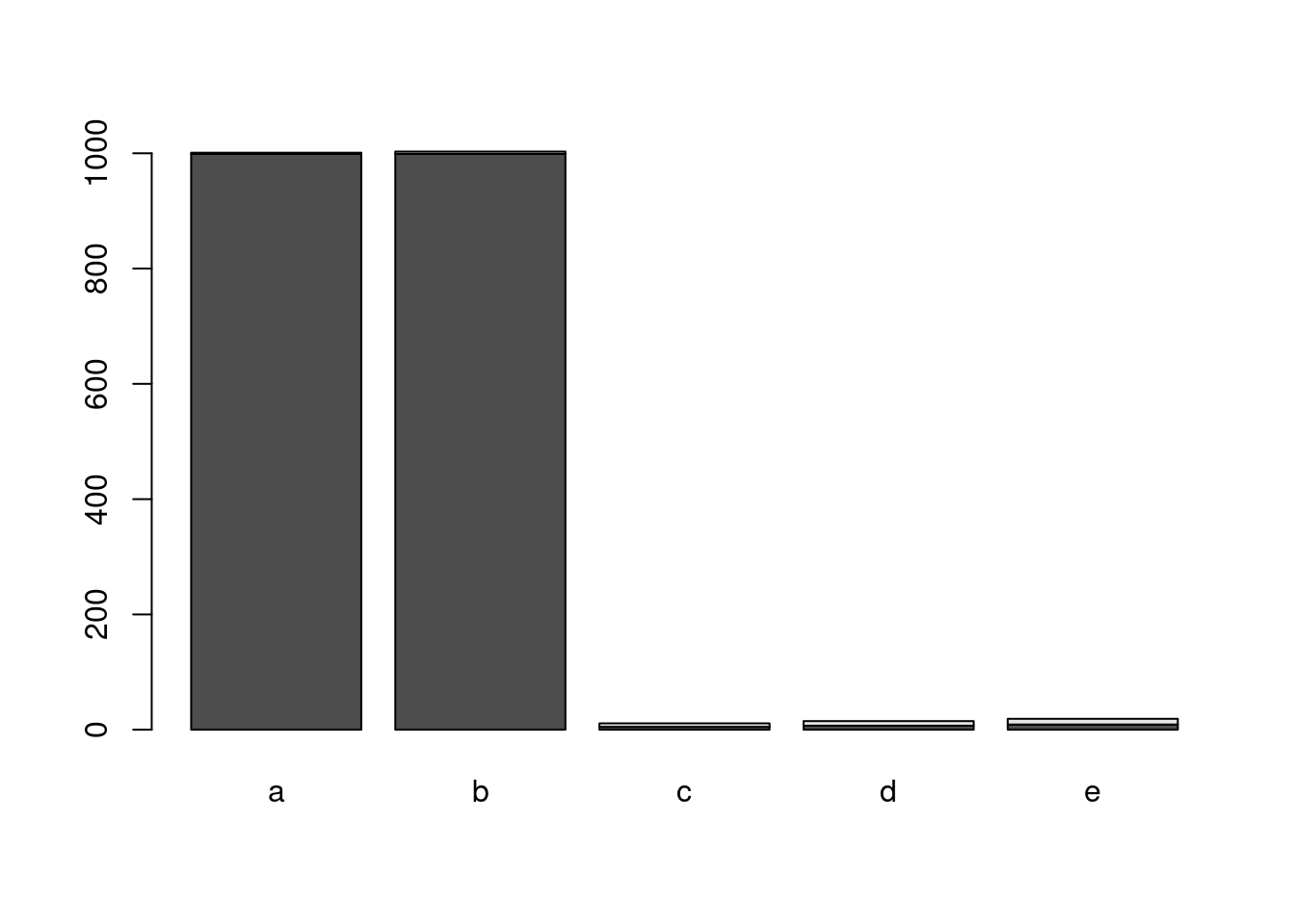
1. `for` loop with append versus inject approach

The following runs a for loop where the result is appended in each iteration with the c() function. The corresponding cbind and rbind for two dimensional data objects would have a similar performance impact as c().

myMA <- matrix(rnorm(1000000), 100000, 10, dimnames=list(1:100000, paste("C", 1:10, sep="")))
results <- NULL
system.time(for(i in seq(along=myMA[,1])) results <- c(results, mean(myMA[i,])))
   user  system elapsed
 39.156   6.369  45.559

Now the for loop is run with an inject approach for storing the results in each iteration.

results <- numeric(length(myMA[,1]))
system.time(for(i in seq(along=myMA[,1])) results[i] <- mean(myMA[i,]))
   user  system elapsed
  1.550   0.005   1.556

As one can see from the output of system.time, the inject approach is 20-50 times faster.

2. `apply` loop versus `rowMeans`

The following performs a row-wise mean calculation on a large matrix first with an apply loop and then with the rowMeans function.

system.time(myMAmean <- apply(myMA, 1, mean))
  user  system elapsed
 1.452   0.005   1.456

system.time(myMAmean <- rowMeans(myMA))
   user  system elapsed
  0.005   0.001   0.006

Based on the results from system.time, the rowMeans approach is over 200 times faster than the apply loop.

3. `apply` loop versus vectorized approach

In this example row-wise standard deviations are computed with an apply loop and then in a vectorized manner.

system.time(myMAsd <- apply(myMA, 1, sd))
   user  system elapsed
  3.707   0.014   3.721
myMAsd[1:4]
        1         2         3         4
0.8505795 1.3419460 1.3768646 1.3005428

system.time(myMAsd <- sqrt((rowSums((myMA-rowMeans(myMA))^2)) / (length(myMA[1,])-1)))
   user  system elapsed
  0.020   0.009   0.028

myMAsd[1:4]
        1         2         3         4
0.8505795 1.3419460 1.3768646 1.3005428

The vector-based approach in the last step is over 200 times faster than the apply loop.

4. Example of fast querying routine applied to a large matrix

(a) Create a sample matrix

The following lfcPvalMA function creates a test matrix containing randomly generated log2 fold changes (LFCs) and p-values (here: pval or FDRs) for variable numbers of samples or test results. In biology this dataset mimics the results of an analysis of differentially expressed genes (DEGs) from several contrasts arranged in a single matrix (or data.frame).

lfcPvalMA <- function(Nrow=200, Ncol=4, stats_labels=c("lfc", "pval")) {
    set.seed(1410)
    assign(stats_labels[1], runif(n = Nrow * Ncol, min = -4, max = 4))
    assign(stats_labels[2], runif(n = Nrow * Ncol, min = 0, max = 1))
    lfc_ma <- matrix(lfc, Nrow, Ncol, dimnames=list(paste("g", 1:Nrow, sep=""), paste("t", 1:Ncol, "_", stats_labels[1], sep=""))) 
    pval_ma <- matrix(pval, Nrow, Ncol, dimnames=list(paste("g", 1:Nrow, sep=""), paste("t", 1:Ncol, "_", stats_labels[2], sep=""))) 
    statsMA <- cbind(lfc_ma, pval_ma)
    return(statsMA[, order(colnames(statsMA))])
}
degMA <- lfcPvalMA(Nrow=200, Ncol=4, stats_labels=c("lfc", "pval"))
dim(degMA)

[1] 200   8

degMA[1:4,] # Prints first 4 rows of DEG matrix generated as a test data set

       t1_lfc    t1_pval    t2_lfc   t2_pval     t3_lfc   t3_pval     t4_lfc   t4_pval
g1 -1.8476368 0.39486484  1.879310 0.7785999  0.1769551 0.9904342  0.1747932 0.9536679
g2  0.2542926 0.04188993 -1.629778 0.6379570 -1.9280792 0.6106041 -2.3599518 0.1950022
g3  3.4703657 0.73881357  2.047794 0.3129176 -3.8891714 0.1508787  3.7811606 0.2560303
g4 -2.8548158 0.99201512 -2.710385 0.1772805  1.0920515 0.2826038  3.9313225 0.5519854

(b) Organize results in `list`

To filter the results efficiently, it is usually best to store the two different stats (here lfc and pval) in separate matrices (here two) where each has the same dimensions and row/column ordering. Note, in this case a list is used to store the two matrices.

degList <- list(lfc=degMA[ , grepl("lfc", colnames(degMA))], pval=degMA[ , grepl("pval", colnames(degMA))])
names(degList)

[1] "lfc"  "pval"

sapply(degList, dim)

     lfc pval
[1,] 200  200
[2,]   4    4

(c) Combinatorial filter

With the above generated data structure of two complementary matrices it is easy to apply combinatorial filtering routines that are both flexible and time-efficient (fast). The following example queries for fold changes of at least 2 (here lfc >= 1 | lfc <= -1) plus p-values of 0.5 or lower. Note, all intermediate and final results are stored in logical matrices. In addition to boolean comparisons, one can apply basic mathematical operations, such as calculating the sum of each cell across many matrices. This returns a numeric matix of integers representing the counts of TRUE values in each position of the considered logical matrices. Subsequently, one can perform summary and filtering routines on these count-based matrices which is convenient when working with large numbers of matrices. All these matrix-to-matrix comparisons are very fast to compute and require zero looping instructions by the user.

queryResult <- (degList$lfc <= 1 | degList$lfc <= -1) & degList$pval <= 0.5 
colnames(queryResult) <- gsub("_.*", "", colnames(queryResult)) # Adjust column names 
queryResult[1:4,]

      t1    t2    t3    t4
g1  TRUE FALSE FALSE FALSE
g2  TRUE FALSE FALSE  TRUE
g3 FALSE FALSE  TRUE FALSE
g4 FALSE  TRUE FALSE FALSE

(d) Extract query results

Retrieve row labels (genes) that match the query from the previous step in each column, and store them in a list.

matchingIDlist <- sapply(colnames(queryResult), function(x) names(queryResult[queryResult[ , x] , x]), simplify=FALSE)
matchingIDlist

$t1
 [1] "g1"   "g2"   "g5"   "g6"   "g11"  "g16"  "g18"  "g19"  "g21"  "g23"  "g24"  "g31"  "g36"  "g37"  "g41"  "g46"  "g60"  "g61"  "g63"  "g70"  "g71"  "g72"  "g75"  "g81"  "g83"  "g84"  "g88"  "g91"  "g97"  "g98" 
[31] "g100" "g102" "g103" "g104" "g110" "g111" "g112" "g113" "g114" "g120" "g121" "g123" "g124" "g126" "g130" "g134" "g135" "g139" "g140" "g145" "g147" "g153" "g157" "g158" "g159" "g160" "g162" "g170" "g171" "g172"
[61] "g173" "g175" "g178" "g183" "g184" "g187" "g190" "g192" "g196" "g199"

$t2
 [1] "g4"   "g5"   "g7"   "g9"   "g10"  "g12"  "g16"  "g23"  "g34"  "g35"  "g39"  "g41"  "g44"  "g46"  "g47"  "g48"  "g49"  "g50"  "g51"  "g52"  "g56"  "g66"  "g75"  "g80"  "g81"  "g85"  "g88"  "g89"  "g90"  "g94" 
[31] "g99"  "g102" "g112" "g115" "g116" "g118" "g119" "g120" "g129" "g144" "g145" "g148" "g152" "g155" "g156" "g160" "g164" "g165" "g167" "g168" "g170" "g172" "g178" "g186" "g187" "g194" "g197"

$t3
 [1] "g3"   "g6"   "g7"   "g9"   "g12"  "g15"  "g23"  "g25"  "g26"  "g27"  "g38"  "g43"  "g52"  "g53"  "g54"  "g58"  "g66"  "g69"  "g72"  "g76"  "g77"  "g80"  "g84"  "g85"  "g86"  "g88"  "g89"  "g90"  "g91"  "g99" 
[31] "g100" "g107" "g110" "g122" "g124" "g125" "g129" "g134" "g139" "g141" "g143" "g144" "g146" "g148" "g154" "g163" "g165" "g171" "g173" "g178" "g180" "g182" "g188" "g190" "g193" "g195"

$t4
 [1] "g2"   "g5"   "g7"   "g8"   "g9"   "g12"  "g13"  "g15"  "g20"  "g21"  "g26"  "g28"  "g30"  "g31"  "g36"  "g37"  "g38"  "g47"  "g63"  "g64"  "g65"  "g67"  "g68"  "g69"  "g76"  "g77"  "g80"  "g85"  "g90"  "g98" 
[31] "g99"  "g101" "g105" "g106" "g120" "g123" "g125" "g126" "g129" "g131" "g134" "g137" "g140" "g143" "g147" "g148" "g153" "g155" "g157" "g165" "g167" "g170" "g171" "g172" "g174" "g175" "g176" "g178" "g181" "g182"
[61] "g188" "g192" "g199"

Return all row labels (genes) that match the above query across a specified number of columns (here 2). Note, the rowSums function is used for this, which performs the row-wise looping internally and extremely fast.

matchingID <- rowSums(queryResult) > 2 
queryResult[matchingID, , drop=FALSE]

        t1    t2    t3    t4
g5    TRUE  TRUE FALSE  TRUE
g7   FALSE  TRUE  TRUE  TRUE
g9   FALSE  TRUE  TRUE  TRUE
g12  FALSE  TRUE  TRUE  TRUE
g23   TRUE  TRUE  TRUE FALSE
g80  FALSE  TRUE  TRUE  TRUE
g85  FALSE  TRUE  TRUE  TRUE
g88   TRUE  TRUE  TRUE FALSE
g90  FALSE  TRUE  TRUE  TRUE
g99  FALSE  TRUE  TRUE  TRUE
g120  TRUE  TRUE FALSE  TRUE
g129 FALSE  TRUE  TRUE  TRUE
g134  TRUE FALSE  TRUE  TRUE
g148 FALSE  TRUE  TRUE  TRUE
g165 FALSE  TRUE  TRUE  TRUE
g170  TRUE  TRUE FALSE  TRUE
g171  TRUE FALSE  TRUE  TRUE
g172  TRUE  TRUE FALSE  TRUE
g178  TRUE  TRUE  TRUE  TRUE

names(matchingID[matchingID])

 [1] "g5"   "g7"   "g9"   "g12"  "g23"  "g80"  "g85"  "g88"  "g90"  "g99"  "g120" "g129" "g134" "g148" "g165" "g170" "g171" "g172" "g178"

As demonstrated in the above query examples, by setting up the proper data structures (here two matrices with same dimensions), and utilizing vectorized (matrix-to-matrix) operations along with R’s built-in row* and col* stats function family (e.g. rowSums) one can design with very little code flexible query routines that also run very time-efficient.

Functions

Function Overview

A very useful feature of the R environment is the possibility to expand existing functions and to easily write custom functions. In fact, most of the R software can be viewed as a series of R functions.

Syntax to define function

myfct <- function(arg1, arg2, ...) { 
    function_body 
}

Syntax to call functions

myfct(arg1=..., arg2=...)

The value returned by a function is the value of the function body, which is usually an unassigned final expression, e.g.: return()

Function Syntax Rules

General

Functions are defined by
1. The assignment with the keyword function
2. The declaration of arguments/variables (arg1, arg2, ...)
3. The definition of operations (function_body) that perform computations on the provided arguments. A function name needs to be assigned to call the function.

Naming

Function names can be almost anything. However, the usage of names of existing functions should be avoided.

Arguments

It is often useful to provide default values for arguments (e.g.: arg1=1:10). This way they don’t need to be provided in a function call. The argument list can also be left empty (myfct <- function() { fct_body }) if a function is expected to return always the same value(s). The argument ... can be used to allow one function to pass on argument settings to another.

Body

The actual expressions (commands/operations) are defined in the function body which should be enclosed by braces. The individual commands are separated by semicolons or new lines (preferred).

Usage

Functions are called by their name followed by parentheses containing possible argument names. Empty parenthesis after the function name will result in an error message when a function requires certain arguments to be provided by the user. The function name alone will print the definition of a function.

Scope

Variables created inside a function exist only for the life time of a function. Thus, they are not accessible outside of the function. To force variables in functions to exist globally, one can use the double assignment operator: <<-

Examples

Define sample function

myfct <- function(x1, x2=5) { 
    z1 <- x1 / x1
    z2 <- x2 * x2
    myvec <- c(z1, z2) 
    return(myvec)
}

Function usage

Apply function to values 2 and 5

myfct(x1=2, x2=5)

[1]  1 25

Run without argument names

myfct(2, 5)

[1]  1 25

Makes use of default value 5

myfct(x1=2)

[1]  1 25

Print function definition (often unintended)

myfct

function (x1, x2 = 5) 
{
    z1 <- x1/x1
    z2 <- x2 * x2
    myvec <- c(z1, z2)
    return(myvec)
}
<bytecode: 0x55c40df48008>

Programming Exercise on Functions: go here ../rprogramming/index.qmd#exercise-1)

Useful Utilities

Debugging Utilities

Several debugging utilities are available for R. They include:

traceback
browser
options(error=recover)
options(error=NULL)
debug

The Debugging in R page provides an overview of the available resources.

Regular Expressions

R’s regular expression utilities work similar as in other languages. To learn how to use them in R, one can consult the main help page on this topic with ?regexp.

String matching with `grep`

The grep function can be used for finding patterns in strings, here letter A in vector month.name.

month.name[grep("A", month.name)]

[1] "April"  "August"

String substitution with `gsub`

Example for using regular expressions to substitute a pattern by another one using a back reference. Remember: single escapes \ need to be double escaped \\ in R.

gsub('(i.*a)', 'xxx_\\1', "virginica", perl = TRUE)

[1] "vxxx_irginica"

Interpreting a Character String as Expression

Some useful examples

Generates vector of object names in session

myfct <- function(x) x^2
mylist <- ls()
n <- which(mylist %in% "myfct")
mylist[n]

[1] "myfct"

Executes entry in position n as expression

get(mylist[n])

function (x) 
x^2

get(mylist[n])(2)

[1] 4

Alternative approach

eval(parse(text=mylist[n]))

function (x) 
x^2

Replacement, Split and Paste Functions for Strings

Selected examples

Substitution with back reference which inserts in this example _ character

x <- gsub("(a)","\\1_", month.name[1], perl=T) 
x

[1] "Ja_nua_ry"

Split string on inserted character from above

strsplit(x,"_")

[[1]]
[1] "Ja"  "nua" "ry"

Reverse a character string by splitting first all characters into vector fields

paste(rev(unlist(strsplit(x, NULL))), collapse="")

[1] "yr_aun_aJ"

Check Integrity of Files

The integrity of files (e.g. after downloading or copying them) can be checked with md5sum (also see checkMD5sums).

library(tools)
(md5 <- as.vector(md5sum(dir(R.home(), pattern = "^COPY", full.names = TRUE))))

[1] "b234ee4d69f5fce4486a80fdaf4a4263"

identical(md5, md5)

[1] TRUE

identical(md5, sub("^b", "z", md5))

[1] FALSE

Time, Date and Sleep

Selected examples

Return CPU (and other) times that an expression used (here ls)

system.time(ls())

   user  system elapsed 
      0       0       0

Return the current system date and time

date()

[1] "Sun Mar 15 16:44:14 2026"

Pause execution of R expressions for a given number of seconds (e.g. in loop)

Sys.sleep(1)

Example

Import of Specific File Lines with Regular Expression

The following example demonstrates the retrieval of specific lines from an external file with a regular expression. First, an external file is created with the cat function, all lines of this file are imported into a vector with readLines, the specific elements (lines) are then retieved with the grep function, and the resulting lines are split into vector fields with strsplit.

cat(month.name, file="zzz.txt", sep="\n")
x <- readLines("zzz.txt")
x[1:6]

[1] "January"  "February" "March"    "April"    "May"      "June"

x <- x[c(grep("^J", as.character(x), perl = TRUE))]
t(as.data.frame(strsplit(x, "u")))

                [,1]  [,2] 
c..Jan....ary.. "Jan" "ary"
c..J....ne..    "J"   "ne" 
c..J....ly..    "J"   "ly"

Calling External Software

External command-line software can be called with the system and system2 functions. The following example calls blastall from R.

system("blastall -p blastp -i seq.fasta -d uniprot -o seq.blastp")

Possibilities for Executing R Scripts

R console

The source command is used for executing an R script from the R console.

source("my_script.R")

Command-line

The Rscript commmand is used to execute an R script from the command-line.

Rscript myscript.R 
./myscript.R # also possible after including a shebang in myscript.R and making it executable

A shebang needs to be included at the beginning of an R script in order to execute it just by typing the name of the script (here ./myscript.R) after making it executable (see here for UNIX-like OSs). The shebang line is optional when executing R scripts from the R console with the source command or with Rscript from the command-line. The shebang of R scripts looks as follows:

#!/usr/bin/env Rscript

Older alternatives for executing R scripts from the command-line are given below.

R CMD BATCH myscript.R # Alternative way 1 
R --slave < myscript.R # Alternative way 2

Passing arguments from command-line to R

Create an R script named test.R with the following content:

myarg <- commandArgs()
print(iris[1:myarg[6], ])

Then run it from the command-line like this:

Rscript test.R 10

In the given example the number 10 is passed on from the command-line as an argument to the R script which is used to return to STDOUT the first 10 rows of the iris sample data. If several arguments are provided, they will be interpreted as one string and need to be split in R with the strsplit function. A more detailed example can be found here.

Building R Packages

This section has been moved to a dedicated tutorial on R package development here.

Programming Exercises

Exercise 1

`for` loop

Task 1.1: Compute the mean of each row in myMA by applying the mean function in a for loop.

myMA <- matrix(rnorm(500), 100, 5, dimnames=list(1:100, paste("C", 1:5, sep="")))
myve_for <- NULL
for(i in seq(along=myMA[,1])) {
    myve_for <- c(myve_for, mean(as.numeric(myMA[i, ])))
}
myResult <- cbind(myMA, mean_for=myve_for)
myResult[1:4, ]

         C1         C2         C3         C4         C5    mean_for
1 -1.202619 -0.1053735 -1.1074995  0.4269033 -1.3932608 -0.67636998
2  1.174138 -0.8991985 -1.2658862  1.0151751 -0.4075398 -0.07666225
3  1.357860 -1.2370991  0.7402124 -1.0277818  0.4851062  0.06365953
4  1.173512 -1.2724114  0.2270477 -1.5421106  0.7484669 -0.13309912

`while` loop

Task 1.2: Compute the mean of each row in myMA by applying the mean function in a while loop.

z <- 1
myve_while <- NULL
while(z <= length(myMA[,1])) {
    myve_while <- c(myve_while, mean(as.numeric(myMA[z, ])))
    z <- z + 1
}
myResult <- cbind(myMA, mean_for=myve_for, mean_while=myve_while)
myResult[1:4, -c(1,2)]

          C3         C4         C5    mean_for  mean_while
1 -1.1074995  0.4269033 -1.3932608 -0.67636998 -0.67636998
2 -1.2658862  1.0151751 -0.4075398 -0.07666225 -0.07666225
3  0.7402124 -1.0277818  0.4851062  0.06365953  0.06365953
4  0.2270477 -1.5421106  0.7484669 -0.13309912 -0.13309912

Task 1.3: Confirm that the results from both mean calculations are identical

all(myResult[,6] == myResult[,7])

[1] TRUE

`apply` loop

Task 1.4: Compute the mean of each row in myMA by applying the mean function in an apply loop

myve_apply <- apply(myMA, 1, mean)
myResult <- cbind(myMA, mean_for=myve_for, mean_while=myve_while, mean_apply=myve_apply)
myResult[1:4, -c(1,2)]

          C3         C4         C5    mean_for  mean_while  mean_apply
1 -1.1074995  0.4269033 -1.3932608 -0.67636998 -0.67636998 -0.67636998
2 -1.2658862  1.0151751 -0.4075398 -0.07666225 -0.07666225 -0.07666225
3  0.7402124 -1.0277818  0.4851062  0.06365953  0.06365953  0.06365953
4  0.2270477 -1.5421106  0.7484669 -0.13309912 -0.13309912 -0.13309912

Avoiding loops

Task 1.5: When operating on large data sets it is much faster to use the rowMeans function

mymean <- rowMeans(myMA)
myResult <- cbind(myMA, mean_for=myve_for, mean_while=myve_while, mean_apply=myve_apply, mean_int=mymean)
myResult[1:4, -c(1,2,3)]

          C4         C5    mean_for  mean_while  mean_apply    mean_int
1  0.4269033 -1.3932608 -0.67636998 -0.67636998 -0.67636998 -0.67636998
2  1.0151751 -0.4075398 -0.07666225 -0.07666225 -0.07666225 -0.07666225
3 -1.0277818  0.4851062  0.06365953  0.06365953  0.06365953  0.06365953
4 -1.5421106  0.7484669 -0.13309912 -0.13309912 -0.13309912 -0.13309912

To find out which other built-in functions for basic calculations exist, type ?rowMeans.

Exercise 2

Custom functions

Task 2.1: Use the following code as basis to implement a function that allows the user to compute the mean for any combination of columns in a matrix or data frame. The first argument of this function should specify the input data set, the second the mathematical function to be passed on (e.g. mean, sd, max) and the third one should allow the selection of the columns by providing a grouping vector.

myMA <- matrix(rnorm(100000), 10000, 10, dimnames=list(1:10000, paste("C", 1:10, sep="")))
myMA[1:2,]

          C1         C2        C3            C4        C5        C6         C7         C8         C9       C10
1  0.1750576 -0.2826930 0.9290137  0.0830523803 1.4113331 -1.221849 -0.4663186  0.6170635 0.58305534 0.1716817
2 -0.8056727  0.1885557 0.4891758 -0.0003536156 0.8356054  1.406484  1.0363437 -0.1351562 0.09596605 0.4551591

myList <- tapply(colnames(myMA), c(1,1,1,2,2,2,3,3,4,4), list) 
names(myList) <- sapply(myList, paste, collapse="_")
myMAmean <- sapply(myList, function(x) apply(myMA[,x], 1, mean))
myMAmean[1:4,]

     C1_C2_C3      C4_C5_C6       C7_C8     C9_C10
1  0.27379276  0.0908453513  0.07537248  0.3773685
2 -0.04264706  0.7472451361  0.45059378  0.2755626
3  0.49411343 -0.4486259202 -0.08519687  1.0929435
4  0.06575562 -0.0007494971  0.07968924 -0.7374505

Exercise 3

Nested loops to generate similarity matrices

Task 3.1: Create a sample list populated with character vectors of different lengths

setlist <- lapply(11:30, function(x) sample(letters, x, replace=TRUE))
names(setlist) <- paste("S", seq(along=setlist), sep="") 
setlist[1:6]

$S1
 [1] "b" "s" "o" "w" "w" "x" "s" "z" "d" "f" "b"

$S2
 [1] "e" "w" "l" "y" "i" "l" "m" "q" "s" "r" "d" "s"

$S3
 [1] "h" "i" "t" "d" "f" "c" "u" "r" "v" "a" "n" "t" "v"

$S4
 [1] "o" "w" "c" "x" "c" "l" "a" "z" "c" "f" "n" "i" "j" "u"

$S5
 [1] "a" "z" "b" "t" "p" "l" "u" "z" "q" "x" "y" "h" "l" "j" "e"

$S6
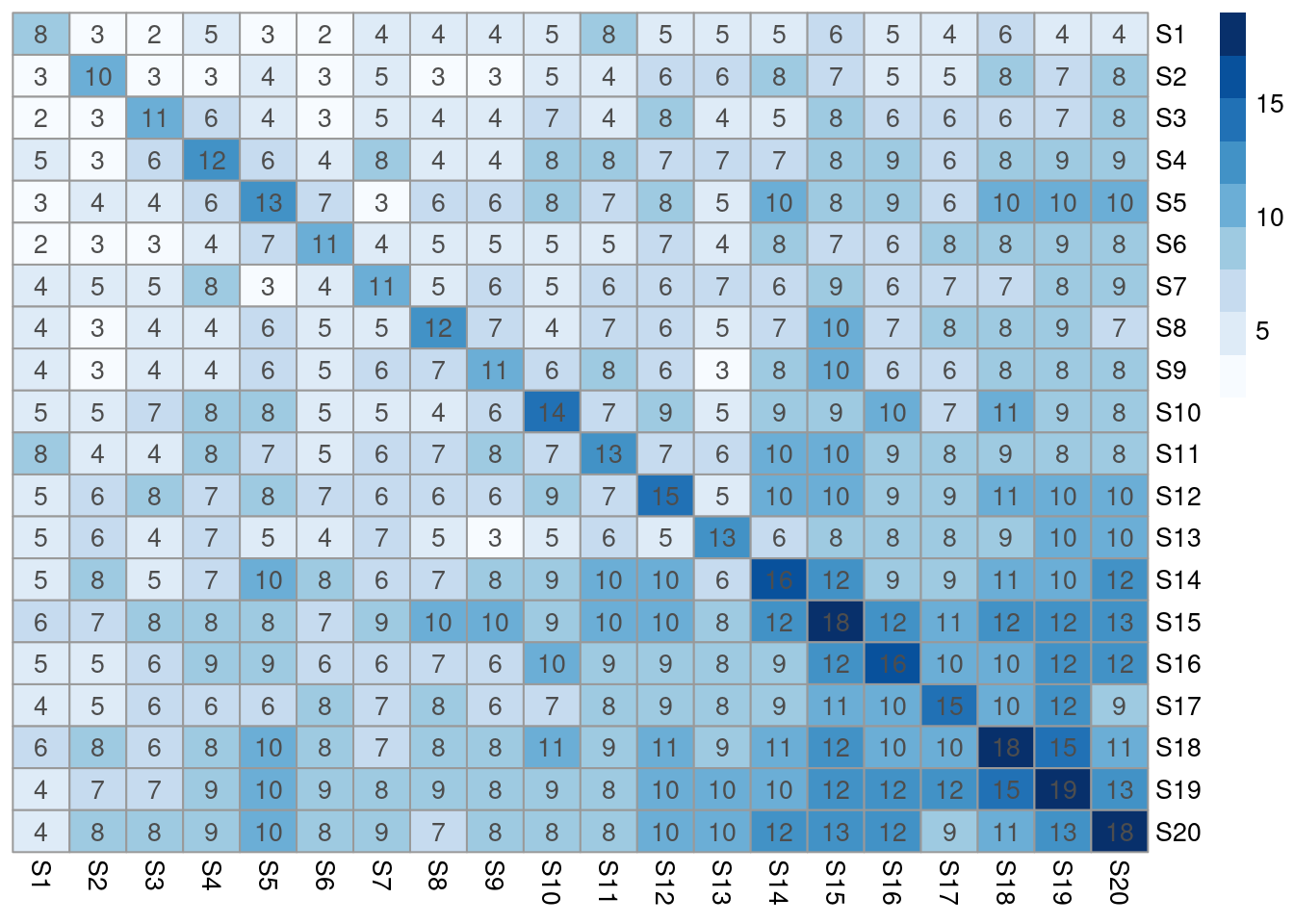
 [1] "z" "v" "n" "v" "b" "m" "p" "p" "z" "g" "l" "j" "z" "z" "t" "e"

Task 3.2: Compute the length for all pairwise intersects of the vectors stored in setlist. The intersects can be determined with the %in% function like this: sum(setlist[[1]] %in% setlist[[2]])

setlist <- sapply(setlist, unique)
olMA <- sapply(names(setlist), function(x) sapply(names(setlist), 
               function(y) sum(setlist[[x]] %in% setlist[[y]])))
olMA[1:12,]

    S1 S2 S3 S4 S5 S6 S7 S8 S9 S10 S11 S12 S13 S14 S15 S16 S17 S18 S19 S20
S1   8  3  2  5  3  2  4  4  4   5   8   5   5   5   6   5   4   6   4   4
S2   3 10  3  3  4  3  5  3  3   5   4   6   6   8   7   5   5   8   7   8
S3   2  3 11  6  4  3  5  4  4   7   4   8   4   5   8   6   6   6   7   8
S4   5  3  6 12  6  4  8  4  4   8   8   7   7   7   8   9   6   8   9   9
S5   3  4  4  6 13  7  3  6  6   8   7   8   5  10   8   9   6  10  10  10
S6   2  3  3  4  7 11  4  5  5   5   5   7   4   8   7   6   8   8   9   8
S7   4  5  5  8  3  4 11  5  6   5   6   6   7   6   9   6   7   7   8   9
S8   4  3  4  4  6  5  5 12  7   4   7   6   5   7  10   7   8   8   9   7
S9   4  3  4  4  6  5  6  7 11   6   8   6   3   8  10   6   6   8   8   8
S10  5  5  7  8  8  5  5  4  6  14   7   9   5   9   9  10   7  11   9   8
S11  8  4  4  8  7  5  6  7  8   7  13   7   6  10  10   9   8   9   8   8
S12  5  6  8  7  8  7  6  6  6   9   7  15   5  10  10   9   9  11  10  10

Task 3.3 Plot the resulting intersect matrix as heat map. The image or the pheatmap functions can be used for this.

library(pheatmap); library("RColorBrewer")
pheatmap(olMA, color=brewer.pal(9,"Blues"), cluster_rows=FALSE, cluster_cols=FALSE, display_numbers=TRUE, number_format="%.0f", fontsize_number=10)

# image(olMA)

Exercise 4

Build your own R package

Task 4.1: Save one or more of your functions to a file called script.R and build the package with the package.skeleton function.

package.skeleton(name="mypackage", code_files=c("script1.R"))

Task 4.2: Build tarball of the package

system("R CMD build mypackage")

Task 4.3: Install and use package

install.packages("mypackage_1.0.tar.gz", repos=NULL, type="source")
library(mypackage)
?myMAcomp # Opens help for function defined by mypackage

Homework 5

See homework section here.

Additional Exercises

Pattern matching and positional parsing of equences

The following sample script patternSearch.R defines functions for importing sequences into R, retrieving reverse and complement of nucleotide sequences, pattern searching, positional parsing and exporting search results in HTML format. Sourcing the script will return usage instructions of its functions.

source("https://raw.githubusercontent.com/tgirke/GEN242/main/content/en/tutorials/rprogramming/scripts/patternSearch.R")

Identify over-represented strings in sequence sets

Example functions for finding over-represented words in sets of DNA, RNA or protein sequences are defined in this script: wordFinder.R. Sourcing the script will return usage instructions of its functions.

source("https://raw.githubusercontent.com/tgirke/GEN242/main/content/en/tutorials/rprogramming/scripts/wordFinder.R")

Object-Oriented Programming (OOP)

R supports several systems for object-oriented programming (OOP). This includes an older S3 system, and the more recently introduced R6 and S4 systems. The latter is the most formal version that supports multiple inheritance, multiple dispatch and introspection. Many of these features are not available in the older S3 system. In general, the OOP approach taken by R is to separate the class specifications from the specifications of generic functions (function-centric system). The following introduction is restricted to the S4 system since it is nowadays the preferred OOP method for package development in Bioconductor. More information about OOP in R can be found in the following introductions:

Define S4 Classes

1. Define S4 Classes with `setClass()` and `new()`

y <- matrix(1:10, 2, 5) # Sample data set
setClass(Class="myclass",
    representation=representation(a="ANY"),
    prototype=prototype(a=y[1:2,]), # Defines default value (optional)
    validity=function(object) { # Can be defined in a separate step using setValidity
        if(class(object@a)[1]!="matrix") {
            return(paste("expected matrix, but obtained", class(object@a)))
        } else {
            return(TRUE)
        }
    }
)

The setClass function defines classes. Its most important arguments are

Class: the name of the class
representation: the slots that the new class should have and/or other classes that this class extends.
prototype: an object providing default data for the slots.
contains: the classes that this class extends.
validity, access, version: control arguments included for compatibility with S-Plus.
where: the environment to use to store or remove the definition as meta data.

2. Create new class instance

The function new creates an instance of a class (here myclass).

myobj <- new("myclass", a=y)
myobj

An object of class "myclass"
Slot "a":
     [,1] [,2] [,3] [,4] [,5]
[1,]    1    3    5    7    9
[2,]    2    4    6    8   10

If evaluated the following would return an error due to wrong input type (data.frame instead of matrix).

new("myclass", a=iris) # Returns error due to wrong input

The arguments of new are:

Class: the name of the class
...: data to include in the new object with arguments according to slots in class definition

3. Initialization method

A more generic way of creating class instances is to define an initialization method (more details below).

setMethod("initialize", "myclass", function(.Object, a) {
    .Object@a <- a/a
    .Object
})
new("myclass", a = y)

An object of class "myclass"
Slot "a":
     [,1] [,2] [,3] [,4] [,5]
[1,]    1    1    1    1    1
[2,]    1    1    1    1    1

4. Usage and helper functions

The ‘@’ operator extracts the contents of a slot. Its usage should be limited to internal functions.

myobj@a

     [,1] [,2] [,3] [,4] [,5]
[1,]    1    3    5    7    9
[2,]    2    4    6    8   10

Create a new S4 object from an old one.

initialize(.Object=myobj, a=as.matrix(cars[1:2,]))

An object of class "myclass"
Slot "a":
  speed dist
1     1    1
2     1    1

If evaluated the removeClass function removes an object from the current session. This does not apply to associated methods.

removeClass("myclass")

5. Inheritance

Inheritance allows to define new classes that inherit all properties (e.g. data slots, methods) from their existing parent classes. The contains argument used below allows to extend existing classes. This propagates all slots of parent classes.

setClass("myclass1", representation(a = "character", b = "character"))
setClass("myclass2", representation(c = "numeric", d = "numeric"))
setClass("myclass3", contains=c("myclass1", "myclass2"))
new("myclass3", a=letters[1:4], b=letters[1:4], c=1:4, d=4:1)

An object of class "myclass3"
Slot "a":
[1] "a" "b" "c" "d"

Slot "b":
[1] "a" "b" "c" "d"

Slot "c":
[1] 1 2 3 4

Slot "d":
[1] 4 3 2 1

getClass("myclass1")

Class "myclass1" [in ".GlobalEnv"]

Slots:
                          
Name:          a         b
Class: character character

Known Subclasses: "myclass3"

getClass("myclass2")

Class "myclass2" [in ".GlobalEnv"]

Slots:
                      
Name:        c       d
Class: numeric numeric

Known Subclasses: "myclass3"

getClass("myclass3")

Class "myclass3" [in ".GlobalEnv"]

Slots:
                                              
Name:          a         b         c         d
Class: character character   numeric   numeric

Extends: "myclass1", "myclass2"

6. Coerce objects to another class

The following defines a coerce method. After this the standard as(..., "...") syntax can be used to coerce the new class to another one.

setAs(from="myclass", to="character", def=function(from) as.character(as.matrix(from@a)))
as(myobj, "character")

 [1] "1"  "2"  "3"  "4"  "5"  "6"  "7"  "8"  "9"  "10"

7. Virtual classes

Virtual classes are constructs for which no instances will be or can be created. They are used to link together classes which may have distinct representations (e.g. cannot inherit from each other) but for which one wants to provide similar functionality. Often it is desired to create a virtual class and to then have several other classes extend it. Virtual classes can be defined by leaving out the representation argument or including the class VIRTUAL as illustrated here:

setClass("myVclass")
setClass("myVclass", representation(a = "character", "VIRTUAL"))

8. Introspection of classes

Useful functions to introspect classes include:

getClass("myclass")
getSlots("myclass")
slotNames("myclass")
extends("myclass2")

Assign Generics and Methods

Generics and methods can be assigned with the methods setGeneric() and setMethod().

1. Accessor functions

This avoids the usage of the @ operator.

setGeneric(name="acc", def=function(x) standardGeneric("acc"))

[1] "acc"

setMethod(f="acc", signature="myclass", definition=function(x) {
    return(x@a)
})
acc(myobj)

     [,1] [,2] [,3] [,4] [,5]
[1,]    1    3    5    7    9
[2,]    2    4    6    8   10

2. Replacement methods

Using custom accessor function with acc <- syntax.

setGeneric(name="acc<-", def=function(x, value) standardGeneric("acc<-"))

[1] "acc<-"

setReplaceMethod(f="acc", signature="myclass", definition=function(x, value) {
                 x@a <- value
                 return(x)
})
## After this the following replace operations with 'acc' work on new object class
acc(myobj)[1,1] <- 999 # Replaces first value
colnames(acc(myobj)) <- letters[1:5] # Assigns new column names
rownames(acc(myobj)) <- letters[1:2] # Assigns new row names
myobj

An object of class "myclass"
Slot "a":
    a b c d  e
a 999 3 5 7  9
b   2 4 6 8 10

Replacement method using [ operator, here [...] <- syntax.

setReplaceMethod(f="[", signature="myclass", definition=function(x, i, j, value) {
                 x@a[i,j] <- value
                 return(x)
})
myobj[1,2] <- 999
myobj

An object of class "myclass"
Slot "a":
    a   b c d  e
a 999 999 5 7  9
b   2   4 6 8 10

3. Behavior of bracket operator

The behavior of the bracket [ subsetting operator can be defined as follows.

setMethod(f="[", signature="myclass",
          definition=function(x, i, j, ..., drop) {
          x@a <- x@a[i,j]
          return(x)
})
myobj[1:2, 1:3] # Standard subsetting works now on new class

An object of class "myclass"
Slot "a":
    a   b c
a 999 999 5
b   2   4 6

4. Print behavior

A convient summary printing behavior for a new class should always be defined.

setMethod(f="show", signature="myclass", definition=function(object) {
          cat("An instance of ", "\"", class(object), "\"", " with ", length(acc(object)[,1]), " elements", "\n", sep="")
          if(length(acc(object)[,1])>=5) {
                print(as.data.frame(rbind(acc(object)[1:2,], ...=rep("...", length(acc(object)[1,])), acc(object)[(length(acc(object)[,1])-1):length(acc(object)[,1]),])))
          } else {
                print(acc(object))
          }
})
myobj # Prints object with custom method

An instance of "myclass" with 2 elements
    a   b c d  e
a 999 999 5 7  9
b   2   4 6 8 10

5. Define custom methods

The following gives an example for defining a data specific method, here randomizing row order of matrix stored in new S4 class.

setGeneric(name="randomize", def=function(x) standardGeneric("randomize"))

[1] "randomize"

setMethod(f="randomize", signature="myclass", definition=function(x) {
          acc(x)[sample(1:length(acc(x)[,1]), length(acc(x)[,1])), ]
})
randomize(myobj)

    a   b c d  e
b   2   4 6 8 10
a 999 999 5 7  9

6. Plotting method

Define a graphical plotting method for new class and allow users to access it with R’s generic plot function.

setMethod(f="plot", signature="myclass", definition=function(x, ...) {
          barplot(as.matrix(acc(x)), ...)
})
plot(myobj)

7. Utilities to inspect methods

Important inspection methods for classes include:

showMethods(class="myclass")
findMethods("randomize")
getMethod("randomize", signature="myclass")
existsMethod("randomize", signature="myclass")

Session Info

sessionInfo()

R version 4.5.1 (2025-06-13)
Platform: x86_64-pc-linux-gnu
Running under: Debian GNU/Linux 11 (bullseye)

Matrix products: default
BLAS:   /usr/lib/x86_64-linux-gnu/blas/libblas.so.3.9.0 
LAPACK: /usr/lib/x86_64-linux-gnu/lapack/liblapack.so.3.9.0  LAPACK version 3.9.0

locale:
 [1] LC_CTYPE=en_US.UTF-8       LC_NUMERIC=C               LC_TIME=en_US.UTF-8        LC_COLLATE=en_US.UTF-8     LC_MONETARY=en_US.UTF-8    LC_MESSAGES=en_US.UTF-8    LC_PAPER=en_US.UTF-8       LC_NAME=C                 
 [9] LC_ADDRESS=C               LC_TELEPHONE=C             LC_MEASUREMENT=en_US.UTF-8 LC_IDENTIFICATION=C       

time zone: America/Los_Angeles
tzcode source: system (glibc)

attached base packages:
[1] tools     stats     graphics  grDevices utils     datasets  methods   base     

other attached packages:
[1] RColorBrewer_1.1-3 pheatmap_1.0.13   

loaded via a namespace (and not attached):
 [1] digest_0.6.39     R6_2.6.1          codetools_0.2-20  fastmap_1.2.0     xfun_0.55         farver_2.1.2      gtable_0.3.6      glue_1.8.0        dichromat_2.0-0.1 knitr_1.51        htmltools_0.5.9   rmarkdown_2.30   
[13] lifecycle_1.0.4   cli_3.6.5         scales_1.4.0      grid_4.5.1        vctrs_0.6.5       compiler_4.5.1    evaluate_1.0.5    yaml_2.3.12       otel_0.2.0        rlang_1.1.6       jsonlite_2.0.0    htmlwidgets_1.6.4

References

Gentleman, Robert. 2008. R Programming for Bioinformatics (Chapman & Hall/CRC Computer Science & Data Analysis). 1 edition. Chapman; Hall/CRC. http://www.amazon.com/Programming-Bioinformatics-Chapman-Computer-Analysis/dp/1420063677.

Overview

Why Programming in R?

R Basics

Code Editors for R

Finding Help

R Scripts

Control Structures

Important Operators

Comparison operators

Logical operators

Conditional Executions: if Statements

Conditional Executions: ifelse Statements

Loops

for loop

Conditional Stop of Loops

while loop

The apply Function Family

apply

tapply

sapply, lapply and vapply

Improving Speed Performance of Loops

1. for loop with append versus inject approach

2. apply loop versus rowMeans

3. apply loop versus vectorized approach

4. Example of fast querying routine applied to a large matrix

(a) Create a sample matrix

(b) Organize results in list

(c) Combinatorial filter

(d) Extract query results

Functions

Function Overview

Function Syntax Rules

Examples

Useful Utilities

Debugging Utilities

Regular Expressions

String matching with grep

String substitution with gsub

Interpreting a Character String as Expression

Replacement, Split and Paste Functions for Strings

Check Integrity of Files

Time, Date and Sleep

Example

Import of Specific File Lines with Regular Expression

Calling External Software

Possibilities for Executing R Scripts

R console

Command-line

Passing arguments from command-line to R

Building R Packages

Programming Exercises

Exercise 1

for loop

while loop

apply loop

Avoiding loops

Exercise 2

Custom functions

Exercise 3

Nested loops to generate similarity matrices

Exercise 4

Build your own R package

Homework 5

Additional Exercises

Pattern matching and positional parsing of equences

Identify over-represented strings in sequence sets

Object-Oriented Programming (OOP)

Define S4 Classes

1. Define S4 Classes with setClass() and new()

2. Create new class instance

3. Initialization method

4. Usage and helper functions

5. Inheritance

6. Coerce objects to another class

7. Virtual classes

8. Introspection of classes

Assign Generics and Methods

1. Accessor functions

2. Replacement methods

3. Behavior of bracket operator

Conditional Executions: `if` Statements

Conditional Executions: `ifelse` Statements

`for` loop

`while` loop

The `apply` Function Family

`apply`

`tapply`

`sapply`, `lapply` and `vapply`

1. `for` loop with append versus inject approach

2. `apply` loop versus `rowMeans`

3. `apply` loop versus vectorized approach

(b) Organize results in `list`

String matching with `grep`

String substitution with `gsub`

`for` loop

`while` loop

`apply` loop

1. Define S4 Classes with `setClass()` and `new()`