Introduction to R
Overview
What is R?
R is a statistical environment and programming language for the analysis and visualization of data. The associated Bioconductor and CRAN package repositories provide many additional R packages for statistical data analysis across a wide array of research areas. The R software is free and runs on all common operating systems.
Why Using R?
- Provides a comprehensive programming language and statistical environment
- Utilizes high-performance data structures and functions optimized for data analysis
- Delivers robust and versatile graphical capabilities
- Integrates with a large ecosystem of analysis packages
- Serves as the leading language for bioinformatics and the industry standard for biostatistics and data mining
- Offers key technical benefits: open-source, free to use, and compatible across all operating systems
Books and Documentation
- Bioinformatics and Computational Biology Solutions Using R and Bioconductor (Gentleman et al., 2005) - URL
- R for Data Science, 2nd ed. (Wickham, Çetinkaya-Rundel & Grolemund, 2023) — The gold standard for learning R with the tidyverse. Covers data import, wrangling, visualization, and modeling. Free to read online and always will be, licensed under CC BY-NC-ND 3.0. URL
- Hands-On Programming with R (Garrett Grolemund) — A friendly introduction to R for non-programmers, covering how to load data, write functions, and use R’s programming tools, with practical data science problems throughout. Free online. URL
- Advanced R, 2nd ed. (Hadley Wickham) — The go-to resource for understanding R deeply: environments, functional programming, metaprogramming, and performance. Free online. URL
- R Programming for Data Science (Roger D. Peng) — Covers R fundamentals with a data science focus, guiding readers through data manipulation, cleaning, and visualization. Suitable for beginners and intermediate users. URL
- Tidy Modeling with R (Kuhn & Silge, 2022) — Covers building, tuning, and evaluating models using the
tidymodelsframework. Free online. URL - Big Book of R (Oscar Baruffa) — A curated directory of 300+ free R books organized by topic (bioinformatics, spatial analysis, machine learning, etc.). Excellent for finding specialized resources. URL
R Working Environments
Examples of R working environments and IDEs with support for syntax highlighting and utilities to send code to the R console:
- RStudio/Posit Desktop: excellent choice for beginners (Cheat Sheets)
- RStudio/Posit Server: web-based UI for RStudio. Available at UCR via onDemand (old standalone web instance will be discontinued).
- RStudio/Posit Cloud: cloud-based RStudio Server
- Nvim-R-Tmux: R working environment based on vim and tmux.
- Emacs (ESS add-on package)
- gedit, Rgedit, RKWard, Eclipse, Tinn-R, Notepad++, NppToR
Example: RStudio
Integrated development environment (IDE) for R. Highly functional for both beginners and advanced users.
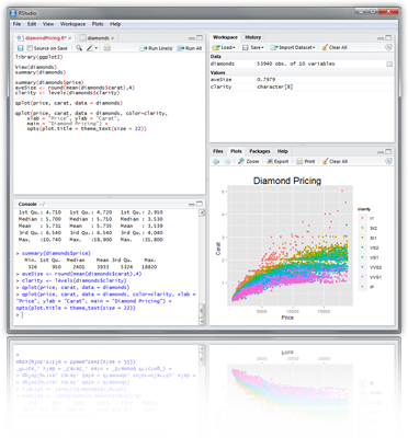
Some userful shortcuts: Ctrl+Enter (send code line), Ctrl+Shift+Enter (send code chunk), Ctrl+Shift+C (comment/uncomment), Ctrl+1/2 (switch window focus)
Example: Nvim-R-Tmux
Terminal-based Working Environment for R: Nvim-R-Tmux.
R Package Repositories
Working routine for tutorials
When working in R, a good practice is to write all commands directly into an R script (qmd or Rmd script), instead of the R console, and then send the commands for execution to the R console with the Ctrl+Enter shortcut in RStudio/Posit, or similar shortcuts in other R coding environments, such as Nvim-R-Tmux. This way all work is preserved and can be reused in the future.
The following instructions in this section provide a short overview of the standard working routine users should use to load R-based tutorials of this website into an R IDE (Nvim-R-Tmux or RStudio). For Nvim-R-Tmux on HPCC users use this install and usage tutorial.
Step 1. Download *.Rmd, qmd or *.R file. These so called source files are always linked on the top right corner of each tutorial. The ones for this tutorial are here. The file download can be accomplished via download.file from within R (see below), wget from the command-line or with the save function in a user’s web browser. The following downloads the qmd file of this tutorial via download.file from the R console.
Load
*.qmd,*.Rmdor*.Rfile in Nvim-R-Tmux or RStudio.Send code from code editor to R console by pressing
Enterin Nvim-R orCtrl + Enterin RStudio. In*.Rmdandqmdfiles the code lines are in so called code chunks and only those ones can be sent to the console. To obtain in Nvim-R-Tmux a connected R session one has to initiate it by pressing the\rfkey combination. For details see here.
Installation of R, RStudio and R Packages
Install R for your operating system from CRAN.
Install RStudio from RStudio.
Install CRAN Packages from R console like this:
- Install Bioconductor packages as follows:
For more details consult the Bioc Install page and BiocManager package.
Instructions for upgrading R and packages to newer versions are given at the end of this tutorial here.
Getting Around
Startup and Closing Behavior
Starting R: The R GUI versions, including RStudio, under Windows and Mac OS X can be opened by double-clicking their icons. Alternatively, one can start it by typing
Rin a terminal (default under Linux).Startup/Closing Behavior: The R environment is controlled by hidden files in the startup directory:
.RData,.Rhistoryand.Rprofile(optional).Closing R:
Save workspace image? [y/n/c]:
- Note: When responding with
y, then the entire R workspace will be written to the.RDatafile which can become very large. Often it is better to selectnhere, because a much better working pratice is to save an analysis protocol to anRorRmdsource file. This way one can quickly regenerate all data sets and objects needed in a future session.
Basic Syntax
Create an object with the assignment operator <- or =
General R command syntax
Instead of the assignment operator one can use the assign function
To simplify chaining of serveral operations, dplyr (magrittr) provides the %>% (pipe) operator, where x %>% f(y) turns into f(x, y). This way one can pipe together multiple operations by writing them from left-to-right or top-to-bottom. This makes for easy to type and readable code. Details on this are provided in the dplyr tutorial here.
Finding help
Load one or more R packages (libraries)
List functions defined by a library
Load library manual (PDF or HTML file)
Execute an R script from within R
Execute an R script from command-line (the first of the three options is preferred)
Data Types
Numeric data
Example: 1, 2, 3, ...
Character data
Example: "a", "b", "c", ...
Complex data
Example: mix of both
Logical data
Example: TRUE of FALSE
Data Objects
Object types
- List of common object types
vectors: ordered collection of numeric, character, complex and logical values.factors: special type vectors with grouping information of its componentsdata.framesincluding modern variantsDataFrame,tibbles, etc.: two dimensional structures with different data typesmatrices: two dimensional structures with data of same typearrays: multidimensional arrays of vectorslists: general form of vectors with different types of elementsfunctions: piece of code- Many more …
- Simple rules for naming objects and their components
- Object, row and column names should not start with a number
- Avoid spaces in object, row and column names
- Avoid special characters like ‘#’
Vectors (1D)
Definition: numeric or character
Factors (1D)
Definition: vectors with grouping information
Matrices (2D)
Definition: two dimensional structures with data of same type
[1] "matrix" "array" [,1] [,2] [,3] [,4] [,5] [,6] [,7] [,8] [,9] [,10]
[1,] 1 2 3 4 5 6 7 8 9 10
[2,] 11 12 13 14 15 16 17 18 19 20 [,1] [,2] [,3] [,4] [,5] [,6] [,7] [,8] [,9] [,10]
[1,] 1 2 3 4 5 6 7 8 9 10[1] "data.frame"Data Frames (2D)
Definition: data.frames are two dimensional objects with data of variable types
Tibbles
Tibbles are a more modern version of data.frames. Among many other advantages, one can see here that tibbles have a nicer printing bahavior. Much more detailed information on this object class is provided in the dplyr/tidyverse manual section.
Note: The above example uses the iris test dataset that is available in every R installation without explicitly importing or loading it. The following examples will often make use of this dataset.
Arrays
Definition: data structure with one, two or more dimensions
Lists
Definition: containers for any object type
Functions
Definition: piece of code
Subsetting of data objects
(1.) Subsetting by positive or negative index/position numbers
(2.) Subsetting by same length logical vectors
 K  L  M  N  O  P  Q  R  S  T  U  V  W  X  Y  Z
11 12 13 14 15 16 17 18 19 20 21 22 23 24 25 26
(3.) Subsetting by field names
(4.) Subset with $ sign: references a single column or list component by its name
Important Utilities
Combining Objects
The c function combines vectors and lists
The cbind and rbind functions can be used to append columns and rows, respecively.
Accessing Dimensions of Objects
Length and dimension information of objects
Accessing Name Slots of Objects
Accessing row and column names of 2D objects
[1] "1" "2" "3" "4" "5" "6" "7" "8"[1] "Sepal.Length" "Sepal.Width" "Petal.Length" "Petal.Width" "Species" Return name field of vectors and lists
Sorting Objects
The function sort returns a vector in ascending or descending order.
The function order returns a sorting index for sorting an object alphanumerically.
[1] 14 9 39 43 42 4 7 23 48 3 30 12Sorting multiple columns
Check differences
To check whether the values in two objects are the same, one can use the == comparison operator. The all function allows to find out whether all values are the same. To check whether two objects are exactly identical, use the identical function.
Operators and Calculations
Comparison Operators
Comparison operators: ==, !=, <, >, <=, >=
Logical operators for boolean operations: AND: &, OR: |, NOT: !
Basic Calculations
To look up math functions, see Function Index here
Reading and Writing External Data
Import of tabular data
Import of a tab-delimited tabular file
Import of Google Sheets. The following example imports a sample Google Sheet from here. Detailed instructions for interacting from R with Google Sheets with the required googlesheets4 package are here.
Import from Excel sheets works well with readxl. For details see the readxl package manual here. Note: working with tab- or comma-delimited files is more flexible and highly preferred for automated analysis workflows.
Additional import functions are described in the readr package section here.
Export of tabular data
Line-wise import
Line-wise export
Export R object
Import R object
Copy and paste into R
On Windows/Linux systems
On Mac OS X systems
Copy and paste from R
On Windows/Linux systems
On Mac OS X systems
Homework 2A
Homework 2A: Object Subsetting Routines and Import/Export
Useful R Functions
Unique entries
Make vector entries unique with unique
Count occurrences
Count occurrences of entries with table
Aggregate data
Compute aggregate statistics with aggregate
Intersect data
Compute intersect between two vectors with %in%
Merge data frames
Join two data frames by common field entries with merge (here row names by.x=0). To obtain only the common rows, change all=TRUE to all=FALSE. To merge on specific columns, refer to them by their position numbers or their column names.
Graphics in R
Advantages
- Powerful environment for visualizing scientific data
- Integrated graphics and statistics infrastructure
- Publication quality graphics
- Fully programmable
- Highly reproducible
- Full LaTeX and Markdown support via
knitrandR markdown - Vast number of R packages with graphics utilities
Documentation for R Graphics
General
- Graphics Task Page - URL
- R Graph Gallery - URL
- R Graphical Manual - URL
- Paul Murrell’s book R (Grid) Graphics - URL
Interactive graphics
Graphics Environments
Viewing and saving graphics in R
- On-screen graphics
- postscript, pdf, svg
- jpeg, png, wmf, tiff, …
Four major graphic environments
- Low-level infrastructure
- R Base Graphics (low- and high-level)
grid: Manual
- High-level infrastructure \begin{itemize}
Base Graphics: Overview
Important high-level plotting functions
plot: generic x-y plottingbarplot: bar plotsboxplot: box-and-whisker plothist: histogramspie: pie chartsdotchart: cleveland dot plotsimage, heatmap, contour, persp: functions to generate image-like plotsqqnorm, qqline, qqplot: distribution comparison plotspairs, coplot: display of multivariant data
Help on graphics functions
?myfct?plot?par
Preferred Object Types
- Matrices and data frames
- Vectors
- Named vectors
Scatter Plots
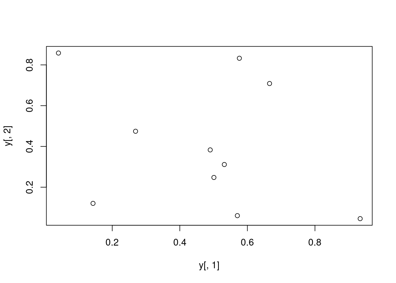
Basic Scatter Plot
Sample data set for subsequent plots
           A          B            C
a 0.26904539 0.47439030 0.4427788756
b 0.53178658 0.31128960 0.3233293493
c 0.93379571 0.04576263 0.0004628517
d 0.14314802 0.12066723 0.4104402000
e 0.57627063 0.83251909 0.9884746270
f 0.49001235 0.38298651 0.8235850153
g 0.66562596 0.70857731 0.7490944304
h 0.50089252 0.24772695 0.2117313873
i 0.57033245 0.06044799 0.8776291364
j 0.04087422 0.85814118 0.1061618729
Plot data
All pairs
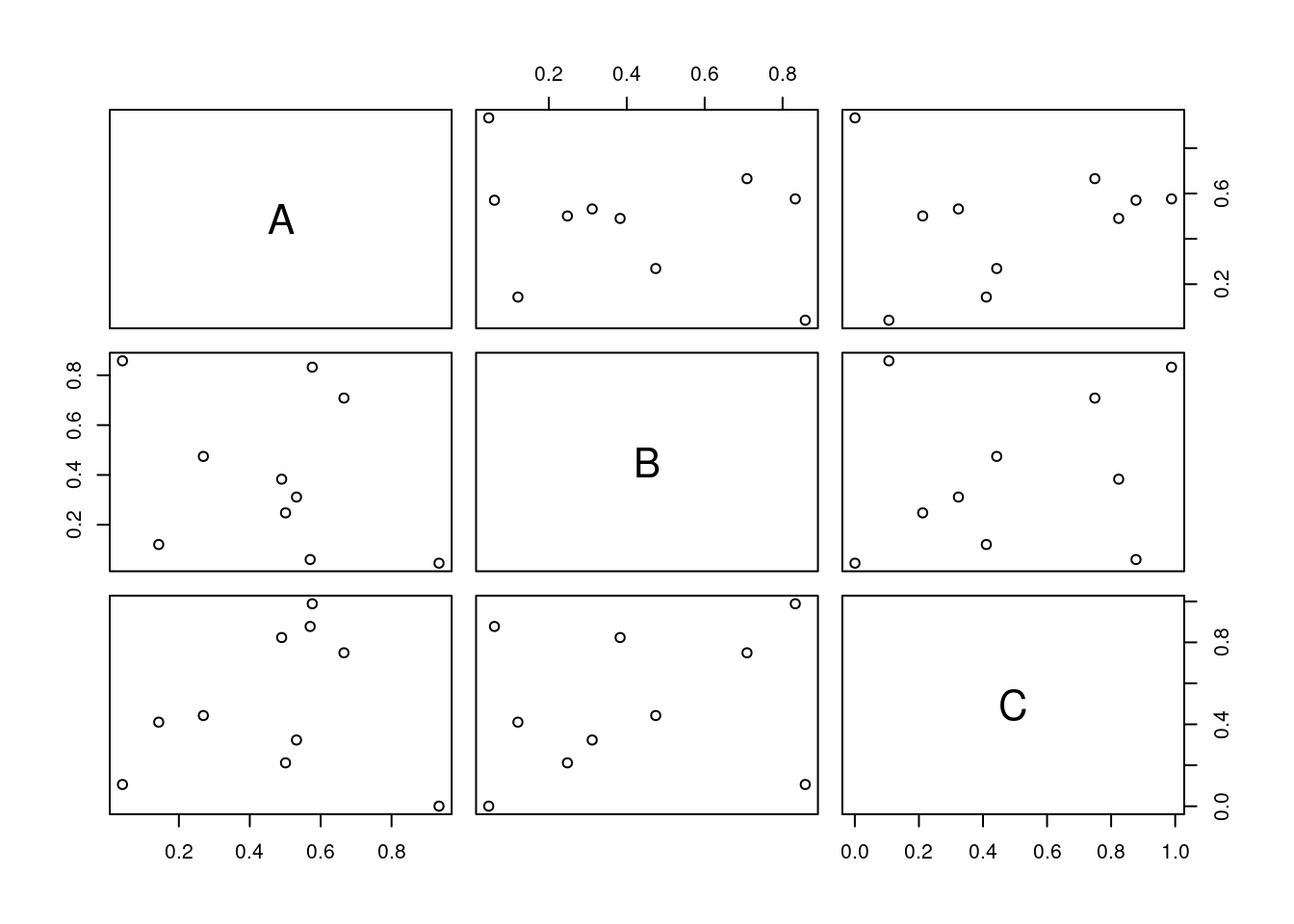
With labels
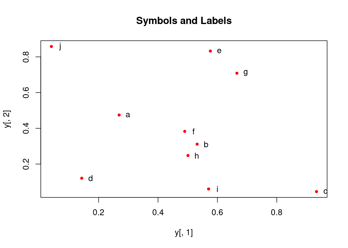
More examples
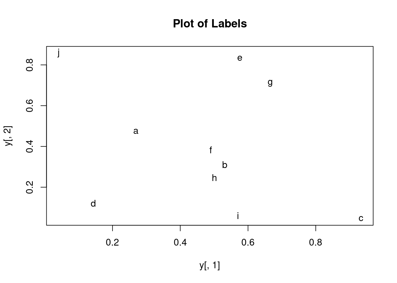
Print instead of symbols the row names
Usage of important plotting parameters
Important arguments
mar: specifies the margin sizes around the plotting area in order:c(bottom, left, top, right)col: color of symbolspch: type of symbols, samples:example(points)lwd: size of symbolscex.*: control font sizes- For details see
?par
Add regression line
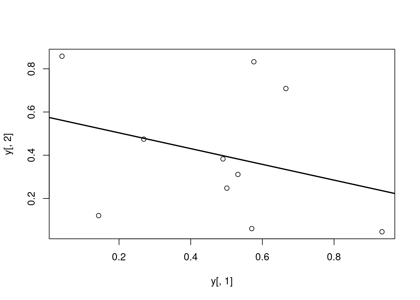
Call:
lm(formula = y[, 2] ~ y[, 1])
Residuals:
Min 1Q Median 3Q Max
-0.40357 -0.17912 -0.04299 0.22147 0.46623
Coefficients:
Estimate Std. Error t value Pr(>|t|)
(Intercept) 0.5764 0.2110 2.732 0.0258 *
y[, 1] -0.3647 0.3959 -0.921 0.3839
---
Signif. codes: 0 '***' 0.001 '**' 0.01 '*' 0.05 '.' 0.1 ' ' 1
Residual standard error: 0.3095 on 8 degrees of freedom
Multiple R-squared: 0.09589, Adjusted R-squared: -0.01712
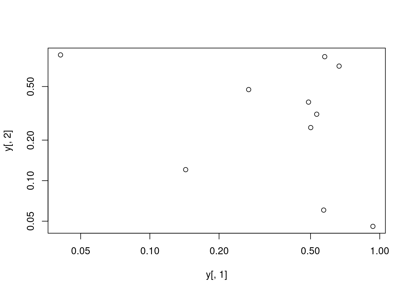
F-statistic: 0.8485 on 1 and 8 DF, p-value: 0.3839Log scale
Same plot as above, but on log scale
Add a mathematical expression
Homework 2B
Homework 2B: Scatter Plots
Line Plots
Single data set
Many Data Sets
Plots line graph for all columns in data frame y. The split.screen function is used in this example in a for loop to overlay several line graphs in the same plot.
Bar Plots
Basics
barplot(y[1:4,], ylim=c(0, max(y[1:4,])+0.3), beside=TRUE, legend=letters[1:4])
text(labels=round(as.vector(as.matrix(y[1:4,])),2), x=seq(1.5, 13, by=1) + sort(rep(c(0,1,2), 4)), y=as.vector(as.matrix(y[1:4,]))+0.04) 
The barplot function has a convenient default behavior when the input data are provided as matrix containing row and column names. The column names are used in the barplot as group labels (here A to C) and the row names as labels for each measurement within a group (here: a to d). When working with a data.frame or tibble, use as.matrix to coerce the input to a matrix; and to populate or change the rownames or colnames slots, use rownames(y) <- ... or colnames(y) <- ..., respectively.
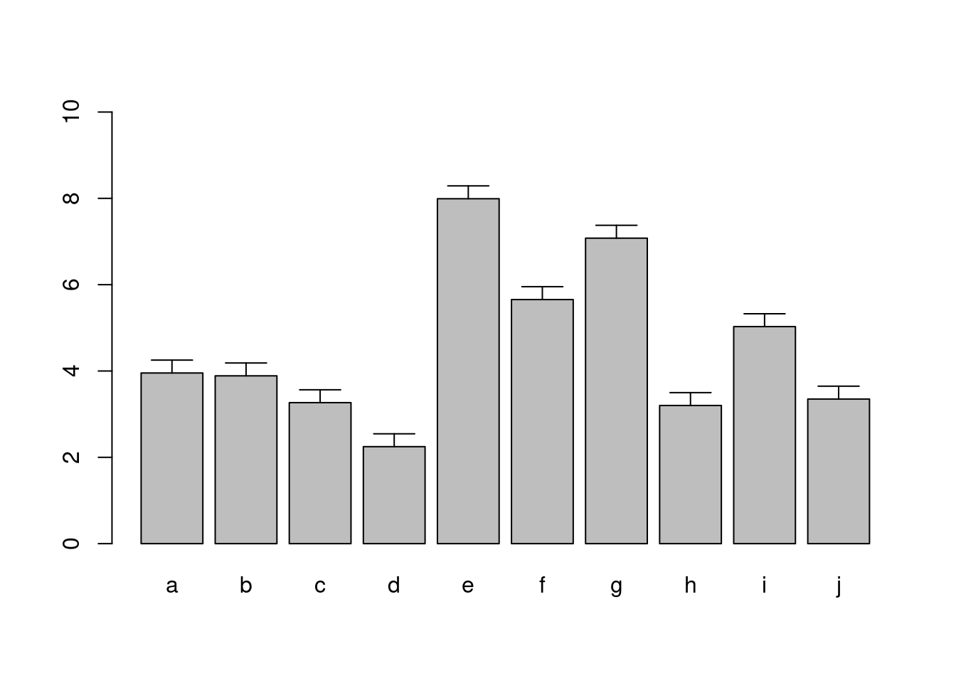
Error Bars
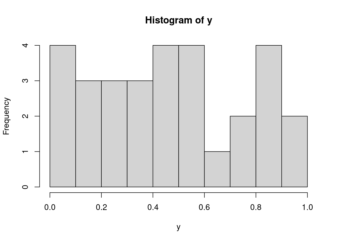
Histograms
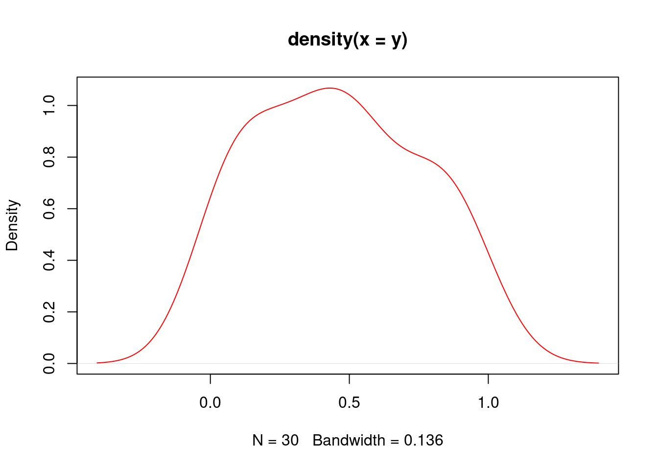
Density Plots
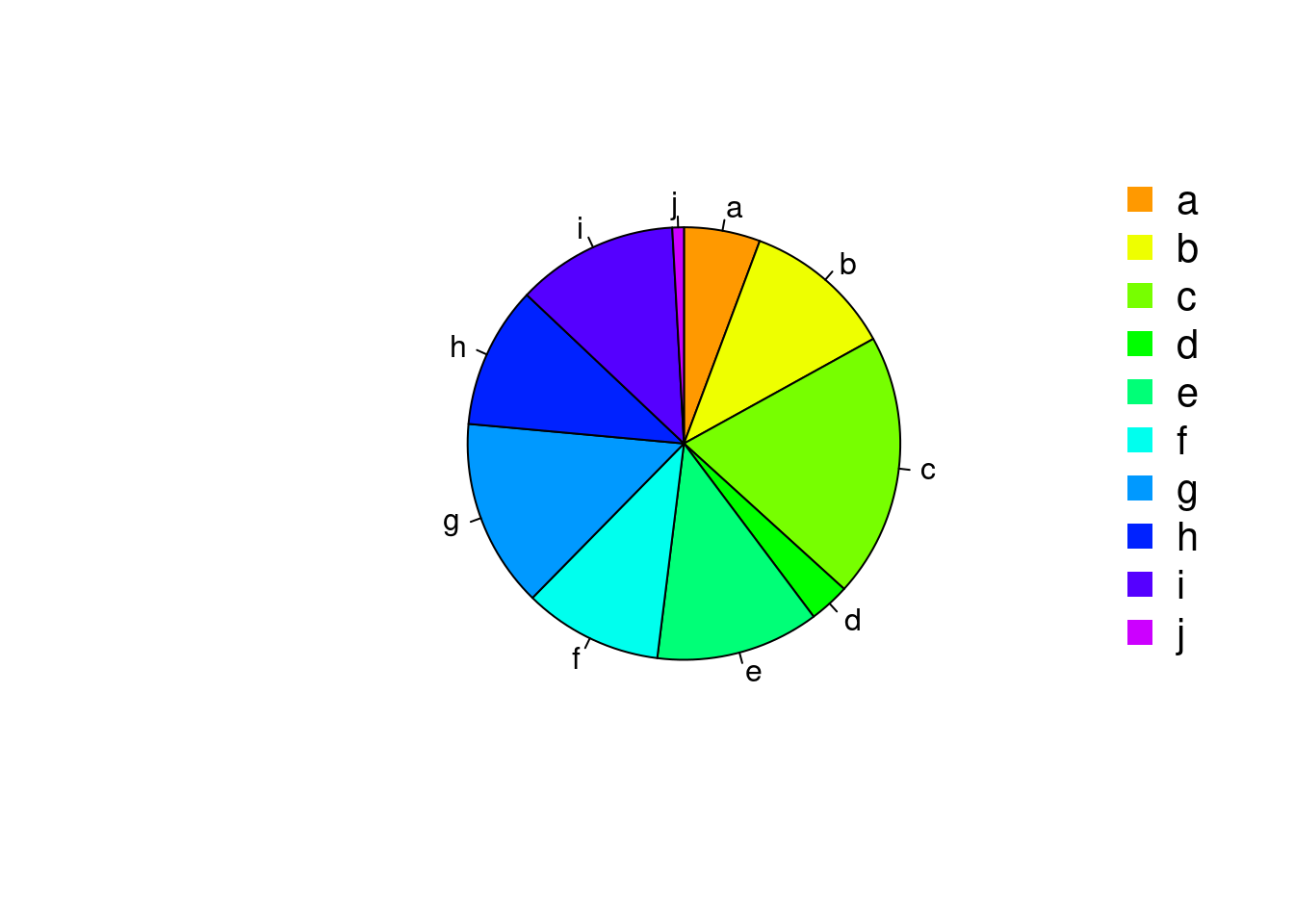
Pie Charts
Color Selection Utilities
Default color palette and how to change it
[1] "black" "#DF536B" "#61D04F" "#2297E6" "#28E2E5" "#CD0BBC" "#F5C710" "gray62" [1] "#FF9900" "#FFBF00" "#FFE600" "#F2FF00" "#CCFF00"The gray function allows to select any type of gray shades by providing values from 0 to 1
Color gradients with colorpanel function from gplots library`
[1] "#00008B" "#808046" "#FFFF00" "#FFFF80" "#FFFFFF"Much more on colors in R see Earl Glynn’s color chart here
Saving Graphics to File
After the pdf() command all graphs are redirected to file test.pdf. Works for all common formats similarly: jpeg, png, ps, tiff, …
Generates Scalable Vector Graphics (SVG) files that can be edited in vector graphics programs, such as InkScape.
Homework 2C
Homework 2C: Bar Plots
Analysis Routine
Overview
The following exercise introduces a variety of useful data analysis utilities in R.
Analysis Routine: Data Import
Step 1: To get started with this exercise, direct your R session to a dedicated workshop directory and download into this directory the following sample tables. Then import the files into Excel and save them as tab delimited text files.
Import the tables into R
Import molecular weight table
Import subcelluar targeting table
Online import of molecular weight table
my_mw <- read.delim(file="https://faculty.ucr.edu/~tgirke/Documents/R_BioCond/Samples/MolecularWeight_tair7.xls", header=TRUE, sep="\t")
my_mw[1:2,]
Online import of subcelluar targeting table
Merging Data Frames
- Step 2: Assign uniform gene ID column titles
- Step 3: Merge the two tables based on common ID field
- Step 4: Shorten one table before the merge and then remove the non-matching rows (NAs) in the merged file
- Homework 2D: How can the merge function in the previous step be executed so that only the common rows among the two data frames are returned? Prove that both methods - the two step version with
na.omitand your method - return identical results. - Homework 2E: Replace all
NAsin the data framemy_mw_target2awith zeros.
Filtering Data
- Step 5: Retrieve all records with a value of greater than 100,000 in ‘MW’ column and ‘C’ value in ‘Loc’ column (targeted to chloroplast).
[1] 170 8- Homework 2F: How many protein entries in the
my_mw_targetdata frame have a MW of greater then 4,000 and less then 5,000. Subset the data frame accordingly and sort it by MW to check that your result is correct.
String Substitutions
- Step 6: Use a regular expression in a substitute function to generate a separate ID column that lacks the gene model extensions.
my_mw_target3 <- data.frame(loci=gsub("\\..*", "", as.character(my_mw_target[,1]), perl = TRUE), my_mw_target)
my_mw_target3[1:3,1:8]- Homework 2G: Retrieve those rows in
my_mw_target3where the second column contains the following identifiers:c("AT5G52930.1", "AT4G18950.1", "AT1G15385.1", "AT4G36500.1", "AT1G67530.1"). Use the%in%function for this query. As an alternative approach, assign the second column to the row index of the data frame and then perform the same query again using the row index. Explain the difference of the two methods.
Calculations on Data Frames
- Step 7: Count the number of duplicates in the loci column with the
tablefunction and append the result to the data frame with thecbindfunction.
- Step 8: Perform a vectorized devision of columns 3 and 4 (average AA weight per protein)
- Step 9: Calculate for each row the mean and standard deviation across several columns
Plotting Example
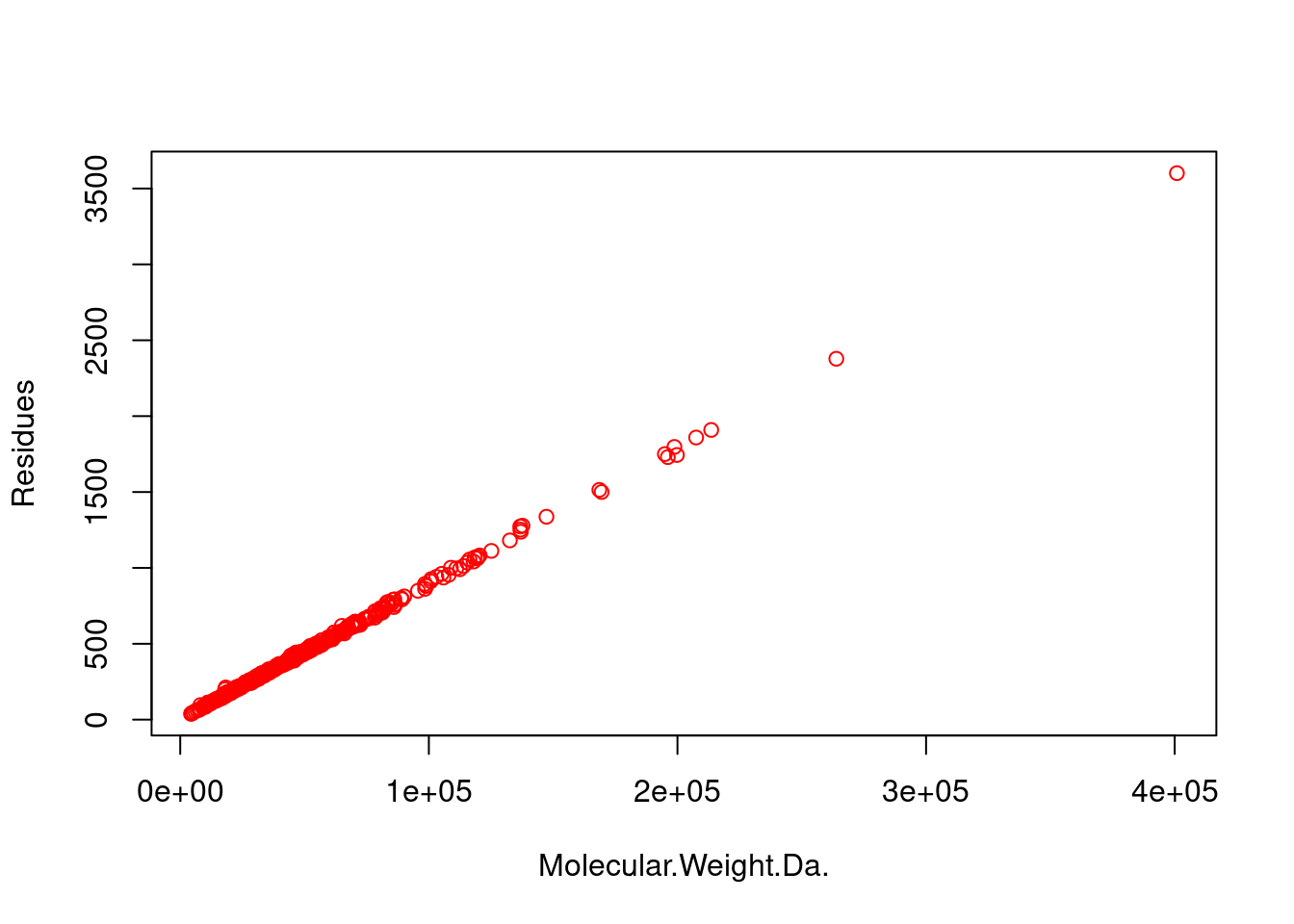
- Step 10: Generate scatter plot for the ‘MW’ and ‘Residues’ columns.
Export Results and Run Entire Exercise as Script
- Step 11: Write the data frame
my_mw_target4into a tab-delimited text file and inspect it in Excel.
- Homework 2H: Write all commands from this exercise into an R script named
exerciseRbasics.R, or download it from here. For demonstration the downloadable script version contains code for generating some additional plots that are not part of this exercise. Then execute the script with thesourcefunction like this:source("exerciseRbasics.R"). This will run all commands of this exercise and generate the corresponding output files in the current working directory. For homework 3H it is not necessary to submit the result files generated by theexerciseRbasics.Rscript. Stating how the script was executed (e.g.sourceorRscriptcommand) will be sufficient.
Or run it from the command-line (not from R!) with Rscript like this:
Miscellaneous Topics
Upgrading to New R/Bioc Versions
When upgrading to a new R version, it is important to understand that a reinstall of all R packages is necessary because CRAN/Bioc packages are developed and tested for specific R versions. This means when upgrading R, then the corresponding packages need to be upgraded to the versions that match the new R version. The following steps will work in many situations.
Step 1. Export a list of all packages installed in a current version of R to a file (below named my_R_pkgs.txt) by running the following commands from within R (or use Rscript -e from command-line)
- Install new version of R, and then from within the new R version all packages one had installed before. The first install command below installs first a series of packages that are useful to have in general no matter what. Custom packages are then installed in the next lines. Note, this can only install packages from CRAN and Bioconductor. Packages from custom sources, including private GitHub accounts, need to be installed separately. Usually, one can identify them by the report generated at the end of the below install routine telling which packages are not available on CRAN or Bioconductor.
Working with Multiple Versions of R
Managing multiple R versions side-by-side can be challenging because standard package managers (apt) or naive source installations overwrite old versions. This guide details how to use rig (R Installation Manager) to sandbox R versions, safely preserve local package libraries, and toggle versions instantly in both Neovim and RStudio.
Why Use rig?
- Zero Compilation: Installs pre-compiled R binaries explicitly built for your Linux distribution in seconds.
- Lightning Fast Packages: Automatically configs CRAN to pull pre-compiled Linux binaries from the Posit Public Package Manager. Installation dropped from hours to seconds.
- Safe Sandbox: Versions are isolated in
/opt/R/and never touch or corrupt base system files.
Installation
Select the tab of the OS you are using and follow the install instructions.
1. Installation (Debian / Ubuntu / ChromeOS)
On Linux systems (including Ubuntu, Debian and ChromeOS penguin containers), install Rig via the official APT repository. Note that the package name is explicitly r-rig.
# 1. Download the cryptographic signing key directly to your trusted directory
sudo wget -O /etc/apt/trusted.gpg.d/rig.gpg https://rig.r-pkg.org/deb/rig.gpg

# 2. Register the accurate sub-repository stream
sudo sh -c 'echo "deb http://rig.r-pkg.org/deb rig main" > /etc/apt/sources.list.d/rig.list'

# 3. Update the package definitions and download the tool
sudo apt update
sudo apt install r-rig
Verify your installation:
2. Managing R Versions with Rig
Adding New Versions
To add R versions side-by-side, use the version number without the R- prefix:
Verifying Installed Versions
Note: Do not use sudo rig system discover. Rig is designed to ignore older, globally pre-existing apt or manual source builds in /usr/lib/R to prevent breaking system libraries.
Creating System Shortcuts
Run this once after installing or adding versions to create the necessary system symbolic links:
This enables version-specific terminal commands like R-4.5.3 and R-4.6.0 globally.
3. Resolving Linux / ChromeOS Path & Alias Conflicts
If typing R in your terminal still launches your old system R version instead of your Rig default, your shell is caching the path or using a hidden system alias. Follow these steps to grant Rig absolute control.
Clear the Shell Cache
Purge Hidden System Aliases
If a system script overrides the R keystroke, add an explicit path priority rule and an un-aliasing safety check to the bottom of your shell profile.
Open your configuration:
Paste these lines at the absolute bottom of the file:
Save and exit, then reload the terminal profile:
4. How Package Libraries Work
Regular User Installations (No Sudo)
Always install your packages as a regular user (without sudo) using standard tools:
Because your user profile does not have write permissions to the /opt/R/ sandbox directories, R automatically routes installations to version-controlled directories inside your home folder: * ~/R/x86_64-pc-linux-gnu-library/4.5/ * ~/R/x86_64-pc-linux-gnu-library/4.6/
Upgrading Safely
If you have an existing directory of user-installed packages from an old installation, Rig will automatically inherit and scan it as long as the major/minor version prefix matches (e.g., 4.5). You can verify your active paths at any time inside your R console using:
5. Handling Future R Version Updates
When a new version of R is released by CRAN, do not use apt upgrade, Homebrew, or standard installers. Standard upgrade paths will overwrite your active environment. Instead, let Rig handle the new release seamlessly.
Step 1: Check for the Latest Available Versions
You can check what versions are available downstream directly from CRAN or Posit’s servers without opening a browser:
Step 2: Install the New Version Side-by-Side
To install the latest release (e.g., 4.6.1), simply run:
Rig will pull the optimized binary package, isolate it in its sandbox (/opt/R/4.6.1 on Linux), and configure its access to fast binary packages automatically. Your old version (4.6.0) remains completely active and untouched.
Step 3: Refresh System Shortcuts
Update your terminal commands so the new version is globally accessible:
This updates the global routes so you can instantly type R-4.6.1 or set it as your new system preference via rig default 4.6.1.
Step 4: What Happens to My Existing Packages?
Because Rig keeps installations fully sandboxed, your new R version will look for a fresh home directory user library matching its exact minor version string (e.g., ~/R/x86_64-pc-linux-gnu-library/4.6/).
- If it’s a patch release (e.g., 4.6.0 to 4.6.1): It shares the same
4.6parent directory! Your new R-4.6.1 installation will instantly see and load all your previously installed packages without you needing to rebuild or reinstall anything. - If it’s a minor/major release (e.g., 4.6.x to 4.7.0): It will look for a new folder (
.../library/4.7/). Because Rig is wired into the Posit Public Package Manager binary repository, runningBiocManager::install()orinstall.packages()to spin up your environment on the new version will finish in seconds.
6. Advanced Workflow: Developing Packages with R-devel
Package developers often need to test code against the upcoming development stream of R (R-devel). Instead of building from source manually, Rig automates downloading, isolating, and refreshing daily development snapshots.
Step 1: Install or Refresh R-devel Natively
To install the latest pre-compiled daily snapshot of R-devel from Posit’s servers:
To pull down fresh updates as the development cycle moves forward, simply repeat the same command. Rig will overwrite the old snapshot in /opt/R/devel/ while leaving your package libraries isolated and intact.
Step 2: Configure Per-Project Local Overrides
Navigate to your R package source directory and set it to target the development environment:
This writes the string devel into a hidden .Rversion file inside your repository workspace.
7. Dynamic Version Discovery in Neovim (init.lua)
To prevent manually editing your Neovim configuration file or relying on special command aliases (like nvim-devel), you can program your editor to read your active Rig configurations on startup.
Add this snippet to your init.lua configuration file. It dynamically scans your working directory for Rig’s local .Rversion tracker and instantly sets up r.vim / Nvim-R to point to the correct language kernel:
-- Dynamically target the active Rig R version path inside Neovim
local local_r_marker = '.Rversion'
local active_r_path = '/usr/local/bin' -- Default fallback path

-- Check if a local Rig configuration file exists in the current folder
local f = io.open(local_r_marker, "r")
if f then
    local assigned_version = f:read("*l") -- Read the string identifier (e.g. "devel", "4.5.3")
    f:close()

    if assigned_version then
        -- Clean up stray whitespaces or return characters
        assigned_version = assigned_version:gsub("%s+", "")
        -- Map to the isolated Rig sandbox path location
        active_r_path = '/opt/R/' .. assigned_version .. '/bin'
    end
end

-- Pass the resolved path directly to your r.vim / Nvim-R plugin configuration
vim.g.R_path = active_r_path
Why this setup is optimal:
- Zero Maintenance: You type
nvimlike normal. - Context-Aware: If your working directory is locked to
rig local devel, Neovim bootsR-devel. If you hop over to an older analytics project locked torig local 4.5.3, it seamlessly mounts4.5.3. - Graceful Fallback: If a project does not have a local envir
On macOS, install Rig using the Homebrew package manager. It automatically provisions architectures for both Intel (x86_64) and Apple Silicon (arm64) natively.
# 1. Install Rig via Homebrew
brew install r-lib/rig/rig

# 2. Configure system paths, symlinks, and permissions
sudo rig system setup
Verify your installation:
2. Managing R Versions
To install R versions side-by-side inside the native macOS framework directory (/Library/Frameworks/R.framework/Versions/):
Verifying Installed Versions
Creating System Shortcuts
This maps version-specific core terminal shortcuts globally (e.g., R-4.5.3).
3. Advantages of Rig on macOS
- Replaces Legacy Tools: It completely replaces old tools like
RSwitch. - Automatic RStudio Binding: When you run
rig default 4.5.3in your Mac terminal, RStudio Desktop automatically binds to that engine the next time it opens. You do not need to manually change any settings inside the RStudio application menus.
4. How Package Libraries Work
Install packages as a standard user without root credentials. R isolates packages cleanly by version strings directly inside your macOS user home directory: * ~/Library/R/arm64/4.5/library (Apple Silicon) * ~/Library/R/x86_64/4.5/library (Intel)
5. Upgrades & R-devel Snapshots
Avoid downloading manual .pkg files from CRAN. Keep your system updated or test packages against the bleeding edge by pulling daily builds directly through the terminal:
Isolate your development repository by typing rig local devel inside your package root folder.
1. Installation
On Windows, install Rig natively using the built-in Windows Package Manager (winget) via an elevated PowerShell or Command Prompt window.
# 1. Install Rig via Winget
winget install R-lib.rig

# 2. Configure system layout (Must run inside an Administrator terminal)
rig system setup
Verify your installation:
2. Managing R Versions
To install R versions side-by-side inside your standard program architecture directory (C:\Program Files\R\):
Verifying Installed Versions
3. Why Rig is Essential on Windows
- Automated Registry Manipulation: Windows tracks default R platforms using complex Registry entries. Whenever you run
rig default <version>, Rig automatically rewrites your Windows Registry keys in the background. - Instant Application Syncing: Third-party software tools (such as RStudio, VS Code, and PowerBI) will instantly discover and swap to your newly active R version without you ever needing to manually modify system Environment Variables or your global
PATH.
4. How Package Libraries Work
Run package commands normally inside your scripts. R blocks writing to protected system directories and maps your assets directly into your personal user directory: * C:\Users\<username>\AppData\Local\R\win-library\4.5\
5. Upgrades & R-devel Snapshots
Do not download manual .exe installers from CRAN. Pull down secure patch adjustments or compiler streams instantly:
Switch your active terminal focus to development test environments using rig local devel inside your package directories.
Usage of rig
Toggling Versions in Neovim (Nvim-R / r.vim)
Neovim relies entirely on your active terminal environment to spin up the R console. Because of this, version toggling with Rig is effortless and zero-config.
Method A: Global Switch (Terminal-wide)
Switch the default R version across your entire system profile:
Any instance of Neovim launched after this command will automatically run R 4.5.3 when triggering the R console (e.g., via \rf).
Method B: Per-Project Local Switch (Recommended)
Navigate to a specific project workspace directory and run:
Rig creates a hidden .Rversion file in that folder. Whenever you cd into this folder and open Neovim, it will seamlessly spin up R 4.5.3 for that project, leaving your global terminal default untouched.
Toggling Versions in RStudio Desktop
RStudio Desktop binds to whatever version of R your terminal points to by default, but it allows users to explicitly lock or choose environments globally or on startup.
Method A: Changing R Version Globally
- Navigate to Tools → Global Options → General → Basic.
- Look for the R version section at the top and click Change…
- Choose Choose a specific version of R.
- Browse and point it directly to the executable inside the Rig sandbox directory:
- For R 4.6.0:
/opt/R/4.6.0/bin/R - For R 4.5.3:
/opt/R/4.5.3/bin/R
- For R 4.6.0:
- Restart RStudio to apply changes.
Note: to toggle the R version in RStudio under Linux, the above menu option is not available. Instead one opens RStudio after selecting the proper R version from the command-line first:
Method B: On-the-Fly Version Selector at Startup
If one needs to frequently hop between versions:
- Close RStudio completely.
- Hold down the Ctrl key on your keyboard while launching RStudio.
- A hidden version selector window will appear before the UI loads. Select your desired environment from the list.
Session Info
R version 4.5.3 (2026-03-11)
Platform: x86_64-pc-linux-gnu
Running under: Debian GNU/Linux 12 (bookworm)

Matrix products: default
BLAS:   /usr/lib/x86_64-linux-gnu/blas/libblas.so.3.11.0
LAPACK: /usr/lib/x86_64-linux-gnu/lapack/liblapack.so.3.11.0  LAPACK version 3.11.0

locale:
 [1] LC_CTYPE=en_US.UTF-8       LC_NUMERIC=C               LC_TIME=en_US.UTF-8        LC_COLLATE=en_US.UTF-8     LC_MONETARY=en_US.UTF-8    LC_MESSAGES=en_US.UTF-8    LC_PAPER=en_US.UTF-8       LC_NAME=C
 [9] LC_ADDRESS=C               LC_TELEPHONE=C             LC_MEASUREMENT=en_US.UTF-8 LC_IDENTIFICATION=C

time zone: America/Los_Angeles
tzcode source: system (glibc)

attached base packages:
[1] stats     graphics  grDevices utils     datasets  methods   base

other attached packages:
 [1] gplots_3.3.0    lubridate_1.9.5 forcats_1.0.1   stringr_1.6.0   dplyr_1.2.0     purrr_1.2.1     readr_2.1.6     tidyr_1.3.2     tibble_3.3.1    tidyverse_2.0.0 ggplot2_4.0.2   limma_3.66.0

loaded via a namespace (and not attached):
 [1] gtable_0.3.6       jsonlite_2.0.0     compiler_4.5.3     gtools_3.9.5       tidyselect_1.2.1   bitops_1.0-9       dichromat_2.0-0.1  scales_1.4.0       yaml_2.3.12        fastmap_1.2.0      statmod_1.5.1
[12] R6_2.6.1           generics_0.1.4     knitr_1.51         htmlwidgets_1.6.4  tzdb_0.5.0         pillar_1.11.1      RColorBrewer_1.1-3 rlang_1.1.7        stringi_1.8.7      xfun_0.56          caTools_1.18.3
[23] S7_0.2.1           otel_0.2.0         timechange_0.4.0   cli_3.6.5          withr_3.0.2        magrittr_2.0.4     digest_0.6.39      grid_4.5.3         hms_1.1.4          lifecycle_1.0.5    vctrs_0.7.1
[34] KernSmooth_2.23-26 evaluate_1.0.5     glue_1.8.0         farver_2.1.2       rmarkdown_2.30     tools_4.5.3        pkgconfig_2.0.3    htmltools_0.5.9