Tidyverse and Some SQLite

Author

Thomas Girke

Published

May 30, 2026

Overview

Modern object classes and methods for handling data.frame like structures are provided by the dplyr (tidyr) and data.table packages. A related example is Bioconductor’s DataTable object class (“Learn the tidyverse,” n.d.). This tutorial provides a short introduction to the usage and functionalities of the dplyr and related packages.

Why learn both base R and tidyverse?

Most genomics and Bioconductor package documentation is written in base R, which is why GEN242 introduces base R syntax first and focuses on it throughout the course. The tidyverse (centered on dplyr, tidyr, and ggplot2) offers an alternative syntax that many find more readable for interactive data exploration, and you will encounter it frequently in online tutorials, Stack Overflow answers, and newer analysis workflows. This tutorial introduces the key dplyr functions side-by-side with their base R equivalents so you can read and write both styles fluently.

A rough comparison of the three main approaches:

Feature	Base R	dplyr / tidyverse	data.table
Learning curve	Moderate	Low–moderate	Steep
Verbosity	More verbose	Concise, readable	Very concise
Performance (large data)	Moderate	Moderate	Excellent
Bioconductor docs	✓ Primary style	Occasionally	Rarely
Pipe-friendly	With `\\|>` (R ≥ 4.1)	Core design	Partial

The data.table package is not covered in depth here, but its fread() function is introduced for fast file import, as it is widely used even in tidyverse workflows.

Installation

The dplyr (tidyr) environment has evolved into an ecosystem of packages. To simplify package management, one can install and load the entire collection via the tidyverse package. For more details on tidyverse see here.

install.packages("tidyverse")

Construct a `tibble` (`tibble`)

library(tidyverse)
as_tibble(iris) # coerce data.frame to tibble tbl

Reading and writing tabular files

While the base R read/write utilities can be used for data.frames, best time performance with the least amount of typing is achieved with the export/import functions from the readr package. For very large files the fread function from the data.table package achieves the best time performance.

Import with `readr`

Import functions provided by readr include:

read_csv(): comma separated (CSV) files
read_tsv(): tab separated files
read_delim(): general delimited files
read_fwf(): fixed width files
read_table(): tabular files where columns are separated by white-space.
read_log(): web log files

Create a sample tab delimited file for import

write_tsv(iris, "iris.txt") # Creates sample file

Import with read_tsv

iris_df <- read_tsv("iris.txt") # Import with read_tsv from readr package
iris_df

To import Google Sheets directly into R, see here.

Fast table import with `fread`

The fread function from the data.table package provides the best time performance for reading large tabular files into R.

library(data.table)
iris_df <- as_tibble(fread("iris.txt")) # Import with fread and conversion to tibble
iris_df

Note: to ignore lines starting with comment signs, one can pass on to fread a shell command for preprocessing the file. The following example illustrates this option.

fread("grep -v '^#' iris.txt")

Export with `readr`

Export functions provided by readr include

write_delim(): general delimited files
write_csv(): comma separated (CSV) files
write_excel_csv(): excel style CSV files
write_tsv(): tab separated files

For instance, the write_tsv function writes a data.frame or tibble to a tab delimited file with much nicer default settings than the base R write.table function.

write_tsv(iris_df, "iris.txt")

Column and row binds

The equivalents to base R’s rbind and cbind are bind_rows and bind_cols, respectively.

bind_cols(iris_df, iris_df)

bind_rows(iris_df, iris_df)

Extract column as vector

The subsetting operators [[ and $can be used to extract from a tibble single columns as vector.

iris_df[[5]][1:12]

 [1] "setosa" "setosa" "setosa" "setosa" "setosa" "setosa" "setosa" "setosa" "setosa" "setosa" "setosa" "setosa"

iris_df$Species[1:12]

 [1] "setosa" "setosa" "setosa" "setosa" "setosa" "setosa" "setosa" "setosa" "setosa" "setosa" "setosa" "setosa"

Important `dplyr` functions

filter() and slice()
arrange()
select() and rename()
distinct()
mutate() and transmute()
summarise()
sample_n() and sample_frac()

Slice and filter functions

Filter function

filter(iris_df, Sepal.Length > 7.5, Species=="virginica")

Base R code equivalent

iris_df[iris_df[, "Sepal.Length"] > 7.5 & iris_df[, "Species"]=="virginica", ]

Including boolean operators

filter(iris_df, Sepal.Length > 7.5 | Sepal.Length < 5.5, Species=="virginica")

Subset rows by position

dplyr approach

slice(iris_df, 1:2)

Base R code equivalent

iris_df[1:2,]

Subset rows by names

Since tibbles do not contain row names, row wise subsetting via the [,] operator cannot be used. However, the corresponding behavior can be achieved by passing to select a row position index obtained by basic R intersect utilities such as match.

Create a suitable test tibble

df1 <- bind_cols(tibble(ids1=paste0("g", 1:10)), as_tibble(matrix(1:40, 10, 4, dimnames=list(1:10, paste0("CA", 1:4)))))
df1

dplyr approach

slice(df1, match(c("g10", "g4", "g4"), ids1))

Base R equivalent

df1_old <- as.data.frame(df1)
rownames(df1_old) <- df1_old[,1]
df1_old[c("g10", "g4", "g4"),]

Sorting with `arrange`

Row-wise ordering based on specific columns

dplyr approach

arrange(iris_df, Species, Sepal.Length, Sepal.Width)

For ordering descendingly use desc() function

arrange(iris_df, desc(Species), Sepal.Length, Sepal.Width)

Base R code equivalent

iris_df[order(iris_df$Species, iris_df$Sepal.Length, iris_df$Sepal.Width), ]

iris_df[order(iris_df$Species, decreasing=TRUE), ]

Select columns with `select`

Select specific columns

select(iris_df, Species, Petal.Length, Sepal.Length)

Select range of columns by name

select(iris_df, Sepal.Length : Petal.Width)

Drop specific columns (here range)

select(iris_df, -(Sepal.Length : Petal.Width))

Change column order with `relocate`

dplyr approach

For details and examples see ?relocate

relocate(iris_df, Species)

Base R code approach

iris[,c(5, 1:4)]

Renaming columns with `rename`

dplyr approach

rename(iris_df, new_col_name = Species)

Base R code approach

colnames(iris_df)[colnames(iris_df)=="Species"] <- "new_col_names"

Obtain unique rows with `distinct`

dplyr approach

distinct(iris_df, Species, .keep_all=TRUE)

Base R code approach

iris_df[!duplicated(iris_df$Species),]

Add columns

`mutate`

The mutate function allows to append columns to existing ones.

mutate(iris_df, Ratio = Sepal.Length / Sepal.Width, Sum = Sepal.Length + Sepal.Width)

`transmute`

The transmute function does the same as mutate but drops existing columns

transmute(iris_df, Ratio = Sepal.Length / Sepal.Width, Sum = Sepal.Length + Sepal.Width)

`bind_cols`

The bind_cols function is the equivalent of cbind in base R. To add rows, use the corresponding bind_rows function.

bind_cols(iris_df, iris_df)

Summarize data

Summary calculation on single column

summarize(iris_df, mean(Petal.Length))

Summary calculation on many columns

summarize(iris_df[,1:4], across(everything(), mean))

Summarize by grouping column

summarize(group_by(iris_df, Species), mean(Petal.Length))

Aggregate summaries

group_by(iris_df, Species) %>% summarize(across(everything(), mean))

Note: group_by does the looping for the user similar to aggregate or tapply.

Merging tibbles

The dplyr package provides several join functions for merging tibbles by a common key column similar to the merge function in base R. These *_join functions include:

inner_join(): returns join only for rows matching among both tibbles
full_join(): returns join for all (matching and non-matching) rows of two tibbles
left_join(): returns join for all rows in first tibble
right_join(): returns join for all rows in second tibble
anti_join(): returns for first tibble only those rows that have no match in the second one

Sample tibbles to illustrate *.join functions.

df1 <- bind_cols(tibble(ids1=paste0("g", 1:10)), as_tibble(matrix(1:40, 10, 4, dimnames=list(1:10, paste0("CA", 1:4)))))
df1

df2 <- bind_cols(tibble(ids2=paste0("g", c(2,5,11,12))), as_tibble(matrix(1:16, 4, 4, dimnames=list(1:4, paste0("CB", 1:4)))))
df2

Inner join

Note: dplyr 1.1.0+ introduced join_by(ids1 == ids2) as an alternative to the by=c("ids1"="ids2") syntax shown here. Both forms work identically; the older named-vector form is used throughout this tutorial as it remains the most common style in existing genomics code.

inner_join(df1, df2, by=c("ids1"="ids2"))

Left join

left_join(df1, df2, by=c("ids1"="ids2"))

Right join

right_join(df1, df2, by=c("ids1"="ids2"))

Full join

full_join(df1, df2, by=c("ids1"="ids2"))

Anti join

anti_join(df1, df2, by=c("ids1"="ids2"))

For additional join options users want to consult the *_join help pages.

Chaining

To simplify chaining of several operations, dplyr uses the %>% operator from magrittr, where x %>% f(y) turns into f(x, y). This way one can pipe together multiple operations by writing them from left-to-right or top-to-bottom. This makes for easy to type and readable code. Since R-4.1.0, a native pipe |> operator is available that works largely the same as %>%. The native pipe requires no package and is the preferred style in modern base R code. Both forms will appear in online examples, so it is helpful to be comfortable with either:

# magrittr pipe (tidyverse style)
iris_df %>% filter(Species == "setosa") %>% nrow()

# Native pipe (base R >= 4.1, no package needed)
iris_df |> filter(Species == "setosa") |> nrow()

The main practical difference is that |> does not support the . placeholder that %>% allows. For the examples in this tutorial the two are interchangeable.

Example 1

Series of data manipulations and export

read_tsv("iris.txt") %>% # Import with read_tsv from readr package
    as_tibble() %>% # Declare to use tibble
    select(Sepal.Length:Species) %>% # Select columns
    filter(Species=="setosa") %>% # Filter rows by some value
    arrange(Sepal.Length) %>% # Sort by some column
    mutate(Subtract=Petal.Length - Petal.Width) # Calculate and append

    # write_tsv("iris.txt") # Export to file, omitted here to show result

Example 2

Series of summary calculations for grouped data (group_by)

iris_df %>% # Declare tibble to use 
    group_by(Species) %>% # Group by species
    summarize(Mean_Sepal.Length=mean(Sepal.Length), 
              Max_Sepal.Length=max(Sepal.Length),
              Min_Sepal.Length=min(Sepal.Length),
              SD_Sepal.Length=sd(Sepal.Length),
              Total=n())

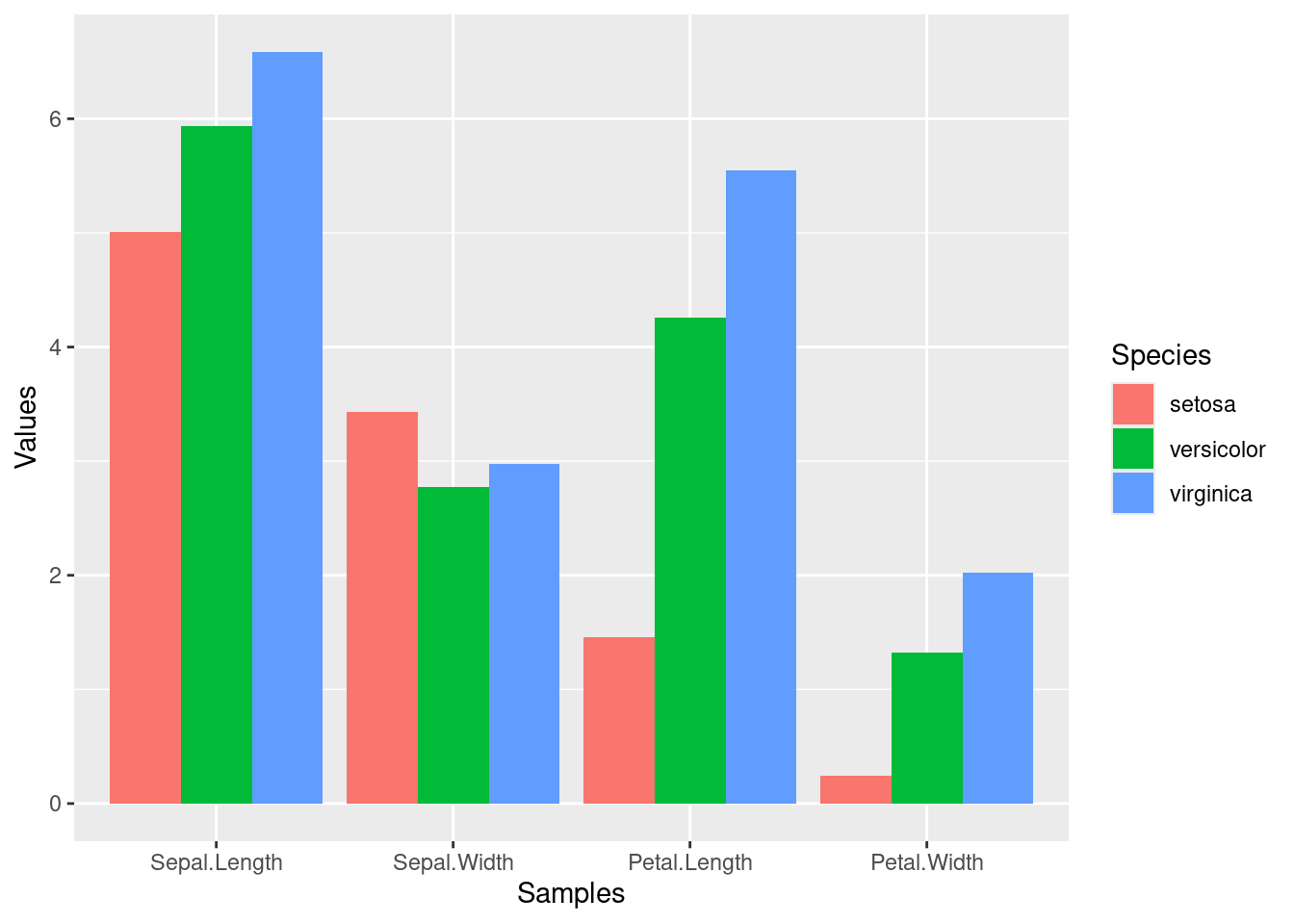
Example 3

Combining dplyr chaining with ggplot

iris_df %>% 
    group_by(Species) %>% 
    summarize(across(everything(), mean)) %>% 
    pivot_longer(cols = -Species, names_to = "Samples", values_to = "Values") %>%
    ggplot(aes(Samples, Values, fill = Species)) + 
            geom_bar(position="dodge", stat="identity")

SQLite Databases

SQLite is a lightweight relational database solution. The RSQLite package provides an easy to use interface to create, manage and query SQLite databases directly from R. Basic instructions for using SQLite from the command-line are available here. A short introduction to RSQLite is available here.

Why SQLite matters in genomics

Many Bioconductor annotation packages — such as org.Hs.eg.db, TxDb.*, and BSgenome companions — store their data internally as SQLite databases. The AnnotationDbi package queries these databases on your behalf, but understanding how SQLite works helps you write more efficient annotation queries, troubleshoot unexpected results, and build your own lightweight databases for project-specific metadata (e.g. sample sheets, gene sets, experimental conditions). The examples below use a small iris-derived database to illustrate the core operations.

Loading data into SQLite databases

The following loads two data.frames derived from the iris data set (here mydf1 and mydf2) into an SQLite database (here test.db).

library(RSQLite)
unlink("test.db") # Delete any existing test.db
mydb <- dbConnect(SQLite(), "test.db") # Creates database file test.db
mydf1 <- data.frame(ids=paste0("id", seq_along(iris[,1])), iris)
mydf2 <- mydf1[sample(seq_along(mydf1[,1]), 10),]
dbWriteTable(mydb, "mydf1", mydf1)
dbWriteTable(mydb, "mydf2", mydf2)

List names of tables in database

dbListTables(mydb)

[1] "mydf1" "mydf2"

Import table into `data.frame`

dbGetQuery(mydb, 'SELECT * FROM mydf2')

Query database

dbGetQuery(mydb, 'SELECT * FROM mydf1 WHERE "Sepal.Length" < 4.6')

Join tables

The two tables can be joined on the shared ids column as follows.

dbGetQuery(mydb, 'SELECT * FROM mydf1, mydf2 WHERE mydf1.ids = mydf2.ids')

Disconnect from database

Always close the database connection when finished to release file locks and flush any pending writes.

dbDisconnect(mydb)

Exercises

The following exercises reinforce the dplyr and SQLite concepts covered in this tutorial. For each dplyr task, try writing the solution in both dplyr and base R syntax.

Exercise 1 — Filtering and sorting
Using the iris dataset, select all rows where Petal.Width > 1.5 and Species is "virginica" or "versicolor". Sort the result by Species (ascending) and then by Petal.Width (descending). Show only the Species, Petal.Length, and Petal.Width columns.

Exercise 2 — Grouped summaries
For each Species in iris, compute the mean and standard deviation of Sepal.Length and Sepal.Width. Store the result as a tibble and inspect it.

Exercise 3 — Mutate and pipe chaining
Using a pipe chain, add a column Petal.Ratio (= Petal.Length / Petal.Width) to iris, filter to rows where Petal.Ratio > 3, and then return only the top 10 rows sorted by Petal.Ratio (descending).

Exercise 4 — Joining tibbles
Create a small annotation tibble:

annot <- tibble(
  Species    = c("setosa", "versicolor", "virginica"),
  CommonName = c("Bristle-pointed iris", "Blue flag iris", "Virginia iris")
)

Join annot to the iris tibble so that every row in iris gains a CommonName column. Which join type is appropriate here, and why?

Exercise 5 — SQLite
Re-open (or re-create) the test.db database from the tutorial. Write an SQL query that returns all rows from mydf1 where Species is "virginica" and Sepal.Length > 6.5. Then write the result back to the database as a new table called virginica_large. Verify the new table exists with dbListTables(), and close the connection when done.

Session Info

sessionInfo()

R version 4.5.3 (2026-03-11)
Platform: x86_64-pc-linux-gnu
Running under: Debian GNU/Linux 12 (bookworm)

Matrix products: default
BLAS:   /usr/lib/x86_64-linux-gnu/blas/libblas.so.3.11.0 
LAPACK: /usr/lib/x86_64-linux-gnu/lapack/liblapack.so.3.11.0  LAPACK version 3.11.0

locale:
 [1] LC_CTYPE=en_US.UTF-8       LC_NUMERIC=C               LC_TIME=en_US.UTF-8        LC_COLLATE=en_US.UTF-8     LC_MONETARY=en_US.UTF-8    LC_MESSAGES=en_US.UTF-8    LC_PAPER=en_US.UTF-8       LC_NAME=C                 
 [9] LC_ADDRESS=C               LC_TELEPHONE=C             LC_MEASUREMENT=en_US.UTF-8 LC_IDENTIFICATION=C       

time zone: America/Los_Angeles
tzcode source: system (glibc)

attached base packages:
[1] stats     graphics  grDevices utils     datasets  methods   base     

other attached packages:
 [1] RSQLite_2.4.6       data.table_1.18.2.1 lubridate_1.9.5     forcats_1.0.1       stringr_1.6.0       dplyr_1.2.0         purrr_1.2.1         readr_2.1.6         tidyr_1.3.2         tibble_3.3.1       
[11] tidyverse_2.0.0     ggplot2_4.0.2       limma_3.66.0       

loaded via a namespace (and not attached):
 [1] generics_0.1.4     stringi_1.8.7      hms_1.1.4          digest_0.6.39      magrittr_2.0.4     evaluate_1.0.5     grid_4.5.3         timechange_0.4.0   RColorBrewer_1.1-3 blob_1.3.0         fastmap_1.2.0     
[12] plyr_1.8.9         jsonlite_2.0.0     DBI_1.2.3          scales_1.4.0       codetools_0.2-20   cli_3.6.5          rlang_1.1.7        crayon_1.5.3       bit64_4.6.0-1      cachem_1.1.0       withr_3.0.2       
[23] yaml_2.3.12        otel_0.2.0         tools_4.5.3        parallel_4.5.3     reshape2_1.4.5     tzdb_0.5.0         memoise_2.0.1      vctrs_0.7.1        R6_2.6.1           lifecycle_1.0.5    htmlwidgets_1.6.4 
[34] bit_4.6.0          vroom_1.7.0        pkgconfig_2.0.3    pillar_1.11.1      gtable_0.3.6       Rcpp_1.1.1         glue_1.8.0         statmod_1.5.1      xfun_0.56          tidyselect_1.2.1   knitr_1.51        
[45] dichromat_2.0-0.1  farver_2.1.2       htmltools_0.5.9    labeling_0.4.3     rmarkdown_2.30     compiler_4.5.3     S7_0.2.1

References

“Learn the tidyverse.” n.d. https://www.tidyverse.org/learn/. https://www.tidyverse.org/learn/.

Overview

Why learn both base R and tidyverse?

Related documentation

Installation

Construct a tibble (tibble)

Reading and writing tabular files

Import with readr

Fast table import with fread

Export with readr

Column and row binds

Extract column as vector

Important dplyr functions

Slice and filter functions

Filter function

Base R code equivalent

Including boolean operators

Subset rows by position

Subset rows by names

Sorting with arrange

Select columns with select

Change column order with relocate

Renaming columns with rename

Obtain unique rows with distinct

Add columns

mutate

transmute

bind_cols

Summarize data

Merging tibbles

Inner join

Left join

Right join

Full join

Anti join

Chaining

Example 1

Example 2

Example 3

SQLite Databases

Why SQLite matters in genomics

Loading data into SQLite databases

List names of tables in database

Import table into data.frame

Query database

Join tables

Disconnect from database

Exercises

Session Info

References

Construct a `tibble` (`tibble`)

Import with `readr`

Fast table import with `fread`

Export with `readr`

Important `dplyr` functions

Sorting with `arrange`

Select columns with `select`

Change column order with `relocate`

Renaming columns with `rename`

Obtain unique rows with `distinct`

`mutate`

`transmute`

`bind_cols`

Import table into `data.frame`