# Install if needed (run once):
# install.packages(c("tidyverse", "caret", "randomForest", "xgboost", "e1071",
#                    "pROC", "pheatmap", "ggrepel", "patchwork", "BiocManager"))
# install.packages(c("treeshap", "shapviz"))   # for SHAP section
# BiocManager::install(c("DESeq2", "curatedTCGAData"))

library(tidyverse)
library(randomForest)
library(xgboost)
library(e1071)
library(pROC)
library(pheatmap)
library(ggrepel)
library(treeshap)
library(shapviz)
library(patchwork)

# Load caret after other packages so caret::train is registered last.
# generics (a DESeq2 dependency) also exports train(); the rule below keeps
# caret::train() as the default throughout this document.
library(caret)
conflictRules("generics", exclude = "train")

# All helper functions are in R/ml_functions.R, organized by method.
source("R/ml_functions.R")Foundations of ML for Genomics
Overview
This tutorial introduces machine learning concepts in the context of genomics using R. We work through a complete ML workflow on a real RNA-Seq time-course dataset: from data preparation and exploration, through model training and comparison, to evaluation and biological interpretation.
Learning objectives:
- Frame a genomics question as a supervised classification problem
- Prepare and split high-dimensional expression data for ML
- Train and compare three classifiers: Random Forest, Gradient Boosting, and SVM
- Evaluate model performance with cross-validation and ROC curves
- Extract and interpret feature importances in a biological context
Setup and Data
Install and load packages
To work with this tutorial, download its qmd file (from here, or use blue QMD button above) as well as the associated R script (from here) that defines the functions used by the qmd script. The R file needs to be stored in a subdirectory named R.
Load example dataset
The RNA-Seq data used in this tutorial is from The Cancer Genome Atlas (TCGA) — specifically primary tumor samples from the BRCA (breast cancer) project, stratified by PAM50 molecular subtype: Basal-like, HER2-enriched, Luminal A, and Luminal B. Data are retrieved via the curatedTCGAData Bioconductor package and cached locally after the first download. The classification task is: predict PAM50 subtype from gene expression.
This is a clinically meaningful question. PAM50 subtyping determines treatment strategy: Basal-like tumors respond to chemotherapy; HER2-enriched to trastuzumab (Herceptin); Luminal A/B to endocrine therapy (tamoxifen, aromatase inhibitors). Standard clinical subtyping requires immunohistochemistry (IHC) staining, which is resource-intensive. RNA-Seq-based prediction is a scalable, cost-effective alternative — and the exact problem that diagnostic ML tools such as Prosigna (PAM50) are built on.
Unlike cross-tissue cancer-type classification (which is trivially easy because tissues have completely different transcriptional programs), subtype classification within a single cancer type is a genuinely hard problem: all four subtypes are breast tumors, and the signal comes from subtle patterns in proliferation, hormone receptor expression, and HER2 amplification. This difficulty produces realistic AUC values (~0.88–0.97) where the three classifiers can be meaningfully compared.
With 75 samples per subtype (~300 total), the dataset is large enough that all three classifiers are fully data-efficient, including XGBoost which needs substantial n.
Note
First run only: load_brca_data() downloads ~50 MB via curatedTCGAData (UQ-normalized RNASeq2GeneNorm assay) and caches to data/brca_subtypes.rds. Subsequent runs load from cache in seconds. Requires: BiocManager::install("curatedTCGAData").
Feature selection (variance filtering)
With ~20,000 genes and ~300 samples, we reduce dimensionality before ML. We keep the top 50 most variable genes (which capture the strongest subtype signal — largely driven by ER/PR expression, HER2 amplification, and proliferation genes) and pad with 450 randomly selected genes from the remainder. This 10% signal / 90% noise ratio makes the classification task realistically challenging while allowing the three algorithms to produce differentiated performance — a better illustration of their relative strengths than a feature set containing only discriminating genes.
Note
In a real analysis one would use all top variable genes without deliberately adding noise. The mixing here is purely pedagogical. On a custom dataset, one can try varying the number of top variable genes (100, 500, 2000) and observe how model performance and feature importance change — this is Exercise 1 below.
feat <- select_features(expr_mat, meta, n_signal = 50, n_noise = 450)
X <- feat$X
y <- feat$y
top_signal <- feat$top_signal
cat("Feature matrix:", nrow(X), "samples x", ncol(X), "features\n")Feature matrix: 288 samples x 500 features Signal genes (top 50 by variance): 50 Noise genes (random): 450 Class distribution:y
Basal  HER2  LumA  LumB
75 63 75 75 Exploratory Analysis
Before fitting any model, always explore your data visually.
PCA of top variable genes
subtype_colors <- c(Basal = "#D62728", HER2 = "#9467BD", LumA = "#1F77B4", LumB = "#FF7F0E")
plot_pca(X, meta, color_values = subtype_colors, color_label = "PAM50 subtype")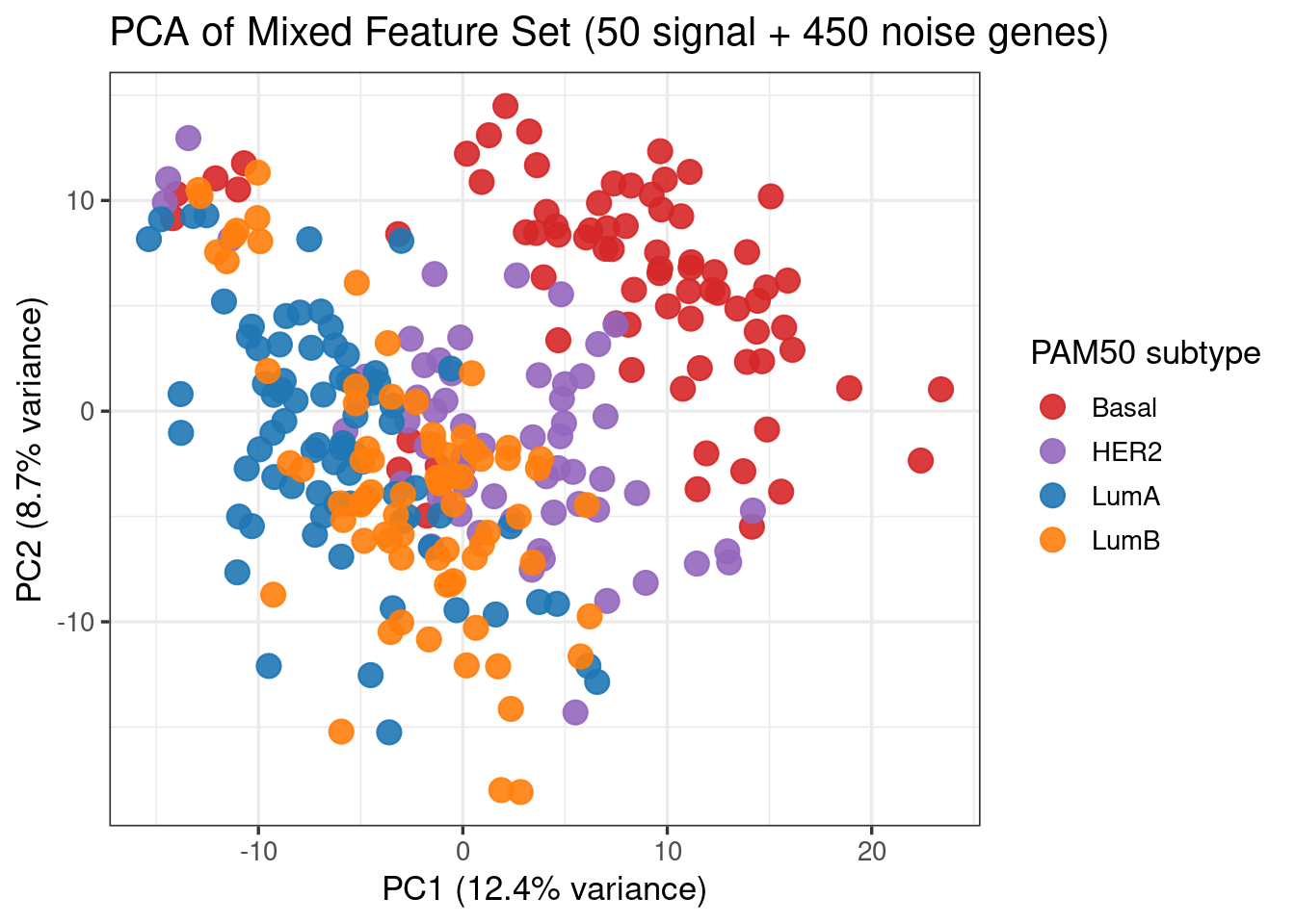
Q: What does Figure 1 tell you about the separability of the classes?
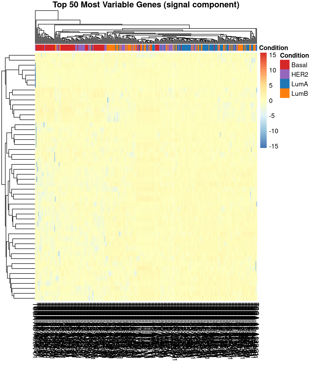
Heatmap of top 50 genes
Data Splitting and Model Comparison Setup
With ~300 samples and balanced classes (~75 per subtype), the BRCA dataset supports a meaningful head-to-head comparison with 5-fold stratified CV — each fold has ~60 samples per class, AUC and mlogloss are well-defined, and XGBoost has enough data to tune its boosting rounds properly.
We additionally generate a simulated dataset (n=200, 500 features, 20 known signal genes) used exclusively to validate feature importance: because the ground truth is known (Gene1–Gene20 carry the signal), we can verify that the models identify the right features. This is not possible on real data where the “true” signal genes are unknown by definition.
sim       <- simulate_data(n_samples = 200, n_features = 500, n_signal = 20)
X_sim     <- sim$X_sim
y_sim     <- sim$y_sim
y_sim_int <- sim$y_sim_int

cat("Simulated dataset:", nrow(X_sim), "samples x", ncol(X_sim), "features\n")
Simulated dataset: 200 samples x 500 featuresClass distribution:y_sim
Case Control
100 100 # 5-fold stratified CV — all classes present in every fold.
ctrl_cv <- make_cv_control(k = 5)
# 0-indexed integer labels for XGBoost multiclass (alphabetical factor level order):
# Basal=0, HER2=1, LumA=2, LumB=3
y_int <- as.integer(y) - 1L
cat("BRCA dataset:", nrow(X), "samples x", ncol(X), "features\n")BRCA dataset: 288 samples x 500 featuresClass distribution:y
Basal HER2 LumA LumB
75 63 75 75 Model Training
We train three classifiers on the BRCA PAM50 dataset (4-class: Basal, HER2, LumA, LumB) and compare them head-to-head. XGBoost uses its native API with the full three-stage workflow; RF and SVM use caret with 5-fold stratified CV.
Random Forest
Random Forest

288 samples
500 predictors
  4 classes: 'Basal', 'HER2', 'LumA', 'LumB'

No pre-processing
Resampling: Cross-Validated (5 fold)
Summary of sample sizes: 230, 231, 231, 230, 230
Resampling results across tuning parameters:

  mtry  logLoss    AUC        prAUC      Accuracy   Kappa      Mean_F1    Mean_Sensitivity  Mean_Specificity  Mean_Pos_Pred_Value  Mean_Neg_Pred_Value  Mean_Precision  Mean_Recall  Mean_Detection_Rate
  10    0.8005832  0.9325441  0.7869094  0.7811857  0.7073985  0.7778149  0.7783974         0.9268383         0.7849606            0.9279567            0.7849606       0.7783974    0.1952964
  22    0.7585447  0.9373682  0.7875626  0.7708409  0.6936286  0.7693349  0.7687179         0.9233499         0.7781776            0.9242164            0.7781776       0.7687179    0.1927102
  50    0.7161214  0.9435015  0.8064028  0.7882638  0.7170766  0.7860411  0.7872436         0.9292709         0.7901832            0.9300656            0.7901832       0.7872436    0.1970659
  Mean_Balanced_Accuracy
  0.8526179
  0.8460339
  0.8582573

AUC was used to select the optimal model using the largest value.
The final value used for the model was mtry = 50.
Gradient Boosting (XGBoost)
XGBoost builds trees sequentially, each correcting the residuals of the previous. It is one of the most widely used ML algorithms in genomics and computational biology, combining speed, regularisation, and strong predictive performance. We use xgboost’s native API directly rather than the caret wrapper, which has compatibility issues with recent xgboost versions.
The standard XGBoost workflow has three stages:
xgb.cvwith early stopping — finds the optimalnroundswithout overfitting- Manual 5-fold CV loop — generates held-out probabilities for an unbiased ROC curve
- Final model on all data — trained with the selected
nroundsfor deployment or feature importance extraction
With n≈300 and balanced classes, all three stages work cleanly on the BRCA data. We run the same workflow a second time on the simulated dataset (below) to validate feature importance against known ground truth.
BRCA subtypes (n ≈ 300, 4-class)
xgb_params <- xgb_params_multiclass(num_class = nlevels(y))

# ── Stage 1: xgb.cv to find optimal nrounds (minimises mlogloss) ──────────────
best_nrounds <- tune_xgb_nrounds(X, y_int, params = xgb_params)
Optimal nrounds: 202 | Best CV MLOGLOSS : 0.5685 # ── Stage 2: 5-fold CV loop — returns n × 4 probability matrix ────────────────
xgb_probs <- xgb_cv_probs(X, y, y_int,
params = xgb_params,
best_nrounds = best_nrounds)
mc_auc <- pROC::auc(pROC::multiclass.roc(y, xgb_probs, quiet = TRUE))
cat("5-fold CV multiclass AUC (XGBoost, BRCA subtypes):", round(mc_auc, 3), "\n")5-fold CV multiclass AUC (XGBoost, BRCA subtypes): 0.945 Simulated dataset (n = 200, feature importance validation)
xgb_params_sim <- xgb_params_large_n()

# ── Stage 1 ────────────────────────────────────────────────────────────────────
best_nrounds_sim <- tune_xgb_nrounds(X_sim, y_sim_int, params = xgb_params_sim)
Optimal nrounds: 63 | Best CV AUC : 0.9513 # ── Stage 2 ────────────────────────────────────────────────────────────────────
xgb_probs_sim <- xgb_cv_probs(X_sim, y_sim, y_sim_int,
params = xgb_params_sim,
best_nrounds = best_nrounds_sim)
# ── Stage 3 ────────────────────────────────────────────────────────────────────
xgb_final_sim <- train_xgb_final(X_sim, y_sim_int,
params = xgb_params_sim,
nrounds = best_nrounds_sim)
imp_sim <- xgboost::xgb.importance(model = xgb_final_sim)
cat("Top 10 features by gain:\n")Top 10 features by gain: Feature Gain Cover Frequency
<char> <num> <num> <num>
1: Gene4 0.12724175 0.10914337 0.08189655
2: Gene11 0.11158230 0.09775866 0.07758621
3: Gene12 0.10698924 0.09322409 0.07327586
4: Gene13 0.09125916 0.08029369 0.06034483
5: Gene17 0.09012926 0.07820066 0.06896552
6: Gene20 0.04953791 0.05045186 0.04741379
7: Gene14 0.04363869 0.03932363 0.03448276
8: Gene18 0.03991159 0.04294176 0.03879310
9: Gene15 0.03441450 0.03329491 0.03017241
10: Gene2 0.03236570 0.02663627 0.03448276xgboost::xgb.plot.importance(imp_sim, top_n = 20,
main = "XGBoost Feature Importance (simulated data)")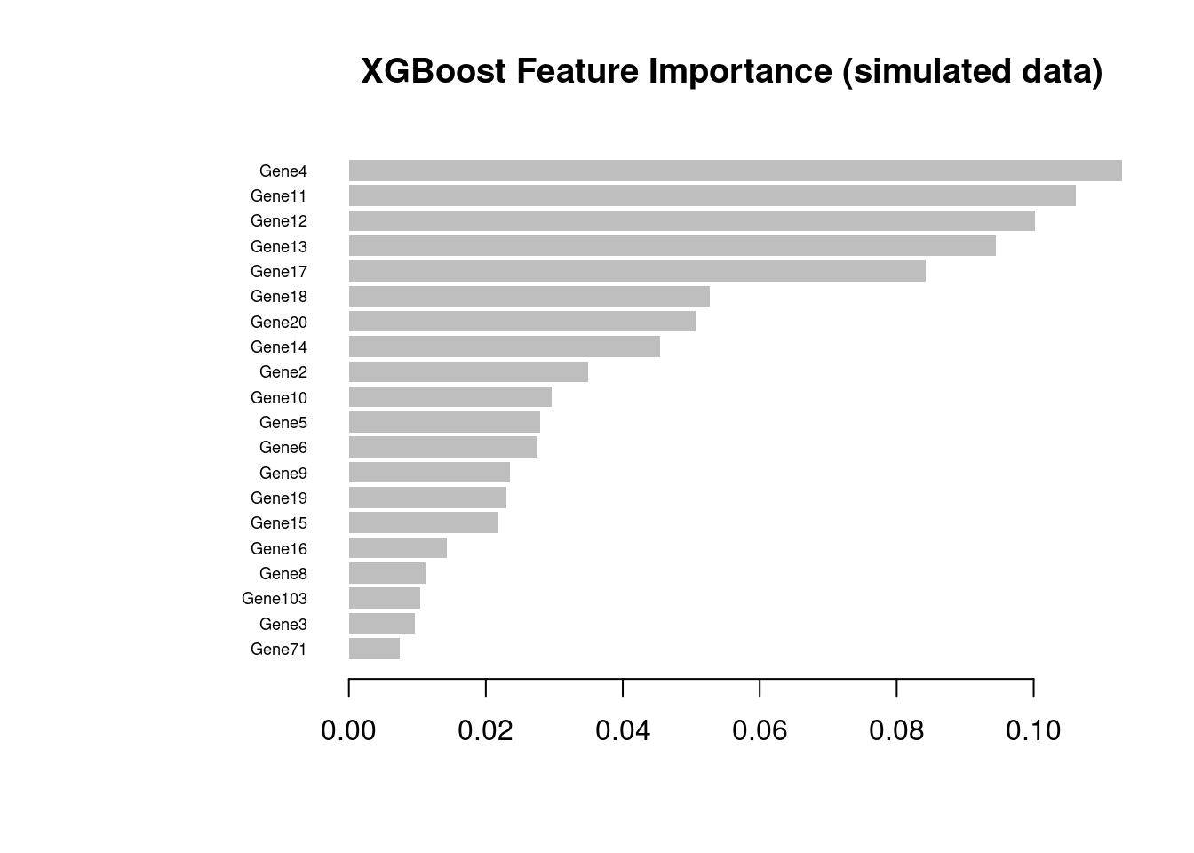
Tip
When using your own dataset: apply this three-stage workflow (xgb.cv → CV probability loop → final model) whenever n > ~50 per class. Key parameters to tune via xgb.cv are max_depth (typically 3–6), eta (0.01–0.1, lower with more rounds), and colsample_bytree (0.3–0.8 for high-dimensional omics data). Use stratified = TRUE in xgb.cv whenever classes are imbalanced.
Support Vector Machine (RBF kernel)
SVMs find a maximum-margin hyperplane in a transformed feature space. The RBF kernel handles nonlinear class boundaries.
Support Vector Machines with Radial Basis Function Kernel

288 samples
500 predictors
  4 classes: 'Basal', 'HER2', 'LumA', 'LumB'

Pre-processing: centered (500), scaled (500)
Resampling: Cross-Validated (5 fold)
Summary of sample sizes: 230, 231, 231, 230, 230
Resampling results across tuning parameters:

  C     logLoss    AUC        prAUC      Accuracy   Kappa      Mean_F1    Mean_Sensitivity  Mean_Specificity  Mean_Pos_Pred_Value  Mean_Neg_Pred_Value  Mean_Precision  Mean_Recall  Mean_Detection_Rate
  0.25  0.7982805  0.8933039  0.6990698  0.6702964  0.5625339  0.6534136  0.6775641         0.8913658         0.6881811            0.8965574            0.6881811       0.6775641    0.1675741
  0.50  0.7398541  0.8987412  0.7133844  0.7120992  0.6163455  0.7054581  0.7140385         0.9043854         0.7204384            0.9064600            0.7204384       0.7140385    0.1780248
  1.00  0.7281491  0.9043735  0.7238571  0.7015729  0.6023019  0.6934770  0.7045513         0.9007900         0.7047473            0.9032612            0.7047473       0.7045513    0.1753932
  2.00  0.7162173  0.9074156  0.7284760  0.7154265  0.6207331  0.7068470  0.7173718         0.9054965         0.7172258            0.9079829            0.7172258       0.7173718    0.1788566
  4.00  0.6895895  0.9146519  0.7363830  0.7465820  0.6621329  0.7434693  0.7483974         0.9158066         0.7458246            0.9165437            0.7458246       0.7483974    0.1866455
  Mean_Balanced_Accuracy
  0.7844650
  0.8092119
  0.8026706
  0.8114341
  0.8321020

Tuning parameter 'sigma' was held constant at a value of 0.001169299
AUC was used to select the optimal model using the largest value.
The final values used for the model were sigma = 0.001169299 and C = 4.
Model Comparison
ROC curves
# Extract n × 4 probability matrices from caret models
subtype_levels <- levels(y)
rf_prob_mat  <- as.matrix(rf_model$pred[order(rf_model$pred$rowIndex), subtype_levels])
svm_prob_mat <- as.matrix(svm_model$pred[order(svm_model$pred$rowIndex), subtype_levels])

roc_all <- plot_roc_multiclass(y, rf_prob_mat, xgb_probs, svm_prob_mat)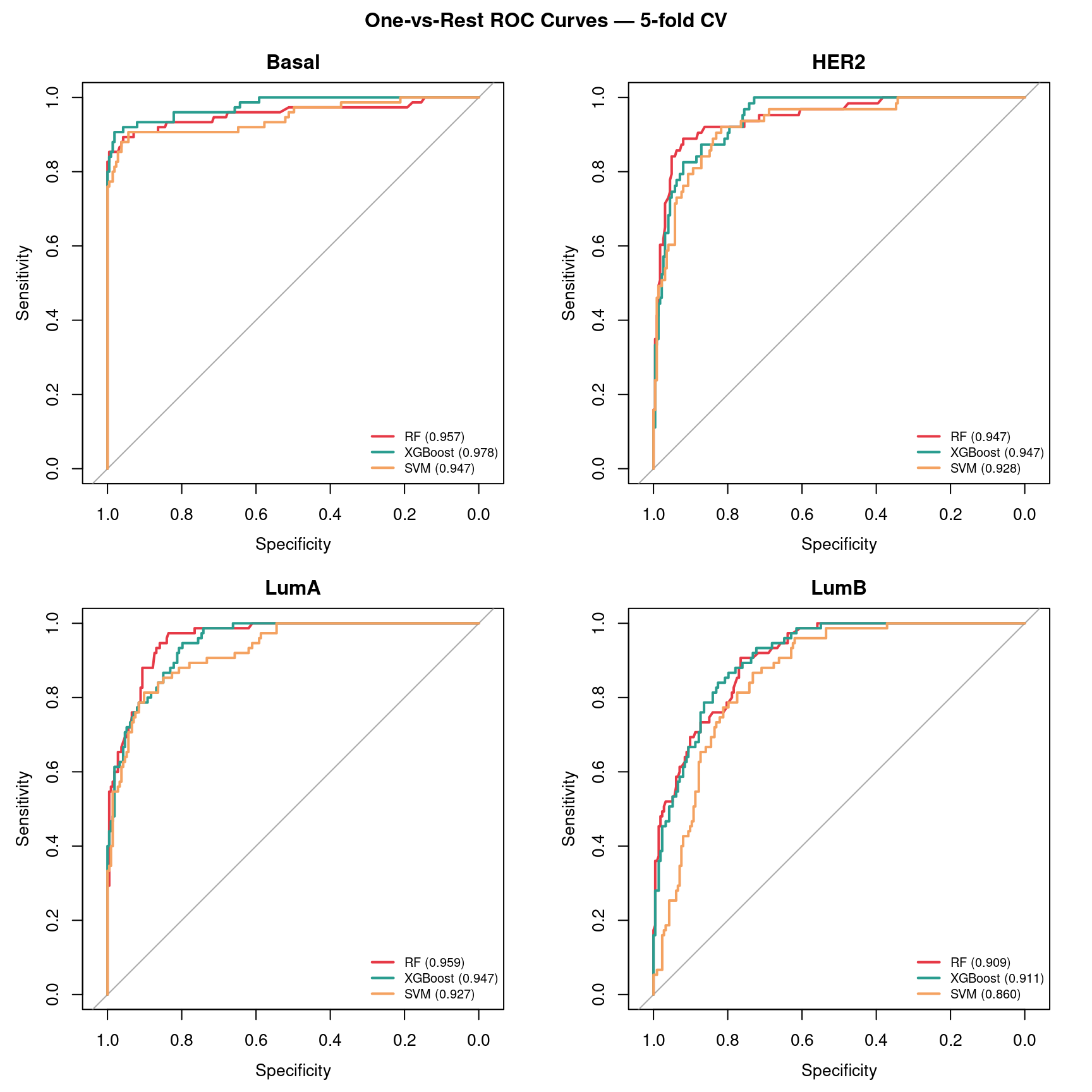
Performance summary
perf_summary <- make_perf_summary(y, rf_prob_mat, xgb_probs, svm_prob_mat,
                                   rf_model, svm_model, best_nrounds)
knitr::kable(perf_summary)| Model | AUC_multiclass | Best_params |
|---|---|---|
| Random Forest | 0.943 | mtry = 50 |
| XGBoost | 0.945 | nrounds = 202 |
| SVM | 0.916 | C = 4 | sigma = 0.0012 |
See Figure 4 for the full ROC curves and Table 1 for the summary.
Interpreting the performance ranking
With n≈300 and 4 balanced classes, all three classifiers have sufficient data to perform well — and the ranking is genuinely competitive. Unlike the small-n regime where RF almost always wins, at this scale XGBoost’s sequential error-correction has enough samples per boosting round to generalize, and may match or exceed RF.
The hardest subtype boundaries are typically LumA vs LumB (both ER+, differ mainly in proliferation rate) and HER2 vs Basal (both ER−, differ in HER2 amplification). The easiest boundary is Basal vs LumA — Basal tumors are triple-negative (ER−, PR−, HER2−) while LumA are strongly ER+, producing a large transcriptional difference. You should see this reflected in the per-subtype AUC panels: Basal one-vs-rest AUC is typically highest (~0.97+), while LumA vs LumB is the weakest.
RF remains a strong baseline due to bagging and random feature subsets that act as implicit regularization (Díaz-Uriarte and Alvarez de Andrés 2006; Qi 2012). SVM with an RBF kernel is competitive when the feature space is well-normalized — as it is here after VST transformation — but tends to be slower to train than tree-based methods at larger n . XGBoost with proper nrounds tuning via xgb.cv can match or surpass RF on well-structured classification problems with sufficient data; in a breast cancer study using TCGA gene expression data, optimized XGBoost achieved the highest AUC among RF, SVM, decision trees, KNN, and logistic regression.
The practical recommendation: use RF as the default baseline — it is robust without tuning and gives competitive results immediately. Invest in XGBoost tuning via xgb.cv when n > ~50 per class and additional performance matters (Chen and Guestrin 2016).
Feature Importance
One of the most useful outputs of ML is knowing which features the model relies on. We validate this on the simulated dataset where ground truth is known (Gene1–Gene20 carry the signal), then examine feature importance on the TCGA data for biological interpretation.
Ground truth validation (simulated data)
# Train RF on simulated data — separate from the BRCA rf_model used for ROC comparison.
rf_model_sim <- train_rf(X_sim, y_sim, ctrl_cv, mtry_grid = c(10, 22, 50))
plot_rf_importance(rf_model_sim, top_n = 20, signal_genes = paste0("Gene", 1:20))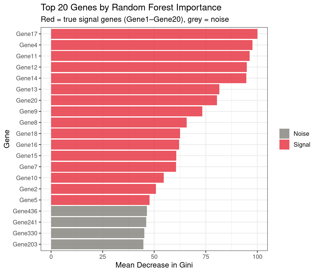
The XGBoost importance plot from the simulated data is shown above (Figure 3). Compare the two rankings: both should recover Gene1–Gene20 in the top positions, confirming that the classifiers have learned the true signal rather than noise.
BRCA data: which genes best distinguish PAM50 subtypes?
imp_brca <- xgboost::xgb.importance(model = xgb_final)
xgboost::xgb.plot.importance(imp_brca, top_n = 20,
                              main = "XGBoost Feature Importance — BRCA PAM50")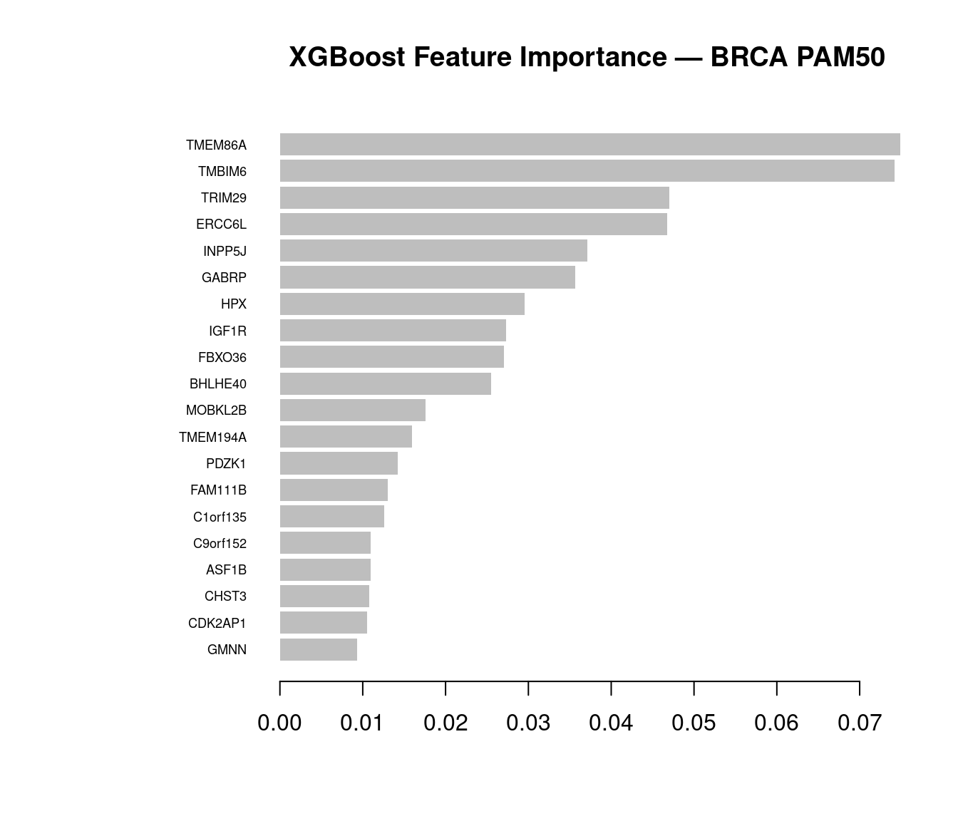
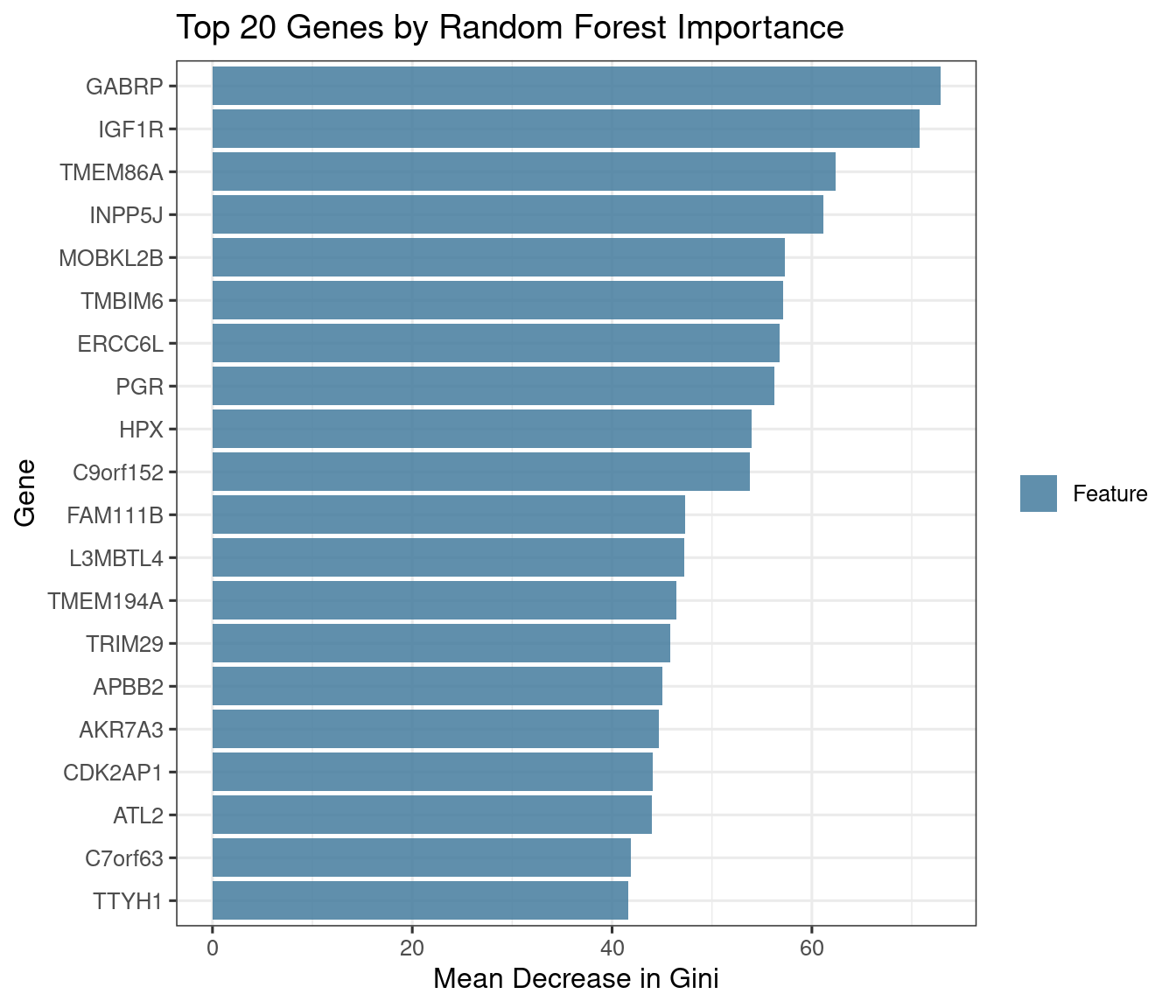
top_rf  <- rownames(rf_model$finalModel$importance)[
             order(rf_model$finalModel$importance[, "MeanDecreaseGini"],
                   decreasing = TRUE)][1:20]
top_xgb <- imp_brca$Feature[1:20]
overlap  <- intersect(top_rf, top_xgb)
cat("RF top-20:  ", paste(top_rf,  collapse = ", "), "\n\n")
RF top-20: GABRP, TMBIM6, TMEM86A, IGF1R, INPP5J, HPX, ERCC6L, C9orf152, PGR, MOBKL2B, TRIM29, FAM111B, AKR7A3, ATL2, DACH1, TMEM194A, L3MBTL4, ASF1B, BHLHE40, BBS4 XGB top-20: TMBIM6, TMEM86A, ERCC6L, GABRP, TRIM29, INPP5J, BHLHE40, FAM111B, FBXO36, HPX, IGF1R, MOBKL2B, C9orf152, TMEM194A, CDK2AP1, PGR, C1orf135, PDZK1, AKR7A3, CHST3 Overlap ( 15 genes): GABRP, TMBIM6, TMEM86A, IGF1R, INPP5J, HPX, ERCC6L, C9orf152, PGR, MOBKL2B, TRIM29, FAM111B, AKR7A3, TMEM194A, BHLHE40 Discussion: The top importance genes are those whose expression profiles differ most consistently across the four PAM50 subtypes. Known subtype markers you should expect to see in one or both rankings:
- ER/PR pathway: ESR1, PGR, FOXA1, GATA3 — high in LumA/LumB, low in Basal
- HER2 amplicon: ERBB2, GRB7, STARD3 — high in HER2, low in others
- Proliferation: MKI67, TOP2A, PCNA — high in Basal and LumB (fast-growing)
- Basal markers: KRT5, KRT14, KRT17 — specific to Basal-like
- Luminal markers: KRT8, KRT18, MLPH — shared by LumA/LumB/HER2
RF vs XGBoost importance — what to expect: RF importance (mean decrease Gini) tends to favour genes with broad, consistent effects across all subtypes. XGBoost gain favours genes that produce the sharpest single splits — often the most extreme subtype contrasts (e.g. a gene that perfectly separates Basal from the rest in one tree node). Genes in the overlap are the most robustly important by both criteria. Genes unique to one ranking are worth investigating: they may reflect the different decision boundaries each algorithm exploits.
SHAP Values
Gini impurity and XGBoost gain tell you which features are globally important across all trees, but not how or why a model made any particular prediction. SHAP (SHapley Additive exPlanations) provides both: for every sample, it assigns each feature a signed contribution (SHAP value) that explains the model’s output relative to a background expectation. Summing all SHAP values for a sample exactly recovers the model’s prediction margin — making SHAP locally faithful, not just globally correlated with importance.
The theoretical foundation is cooperative game theory. SHAP values are Shapley values: the unique solution satisfying four axioms (efficiency, symmetry, dummy, additivity) that fairly distribute the prediction “credit” across features (Lundberg et al. 2020). This makes SHAP the only importance measure that is both locally faithful (per-sample) and globally consistent (rankings do not contradict local effects).
For tree-based models, TreeSHAP computes exact Shapley values in polynomial time (Lundberg2020?), making it practical for the ~300 × 500 matrices used here.
Note
Key distinction from Gini / gain: Gini and gain are by-products of the tree-building algorithm — they measure how much a gene was used to reduce impurity across all training trees. SHAP values measure how much a gene shifts the model’s output for a specific sample. A gene can have high Gini importance (used in many splits) but small SHAP values if those splits produce offsetting positive and negative effects across the population.
Computing TreeSHAP
# TreeSHAP computation (~1-2 min for n=300, p=500)
sv_xgb <- compute_shap_xgb(xgb_final, X)
sv_rf  <- compute_shap_rf(rf_model, X)

# For multiclass XGBoost, shapviz returns one set of SHAP values per class (mshapviz).
# For multiclass RF, treeshap returns a single combined matrix (plain shapviz).
cat("XGBoost SHAP object type:", class(sv_xgb), "\n")
XGBoost SHAP object type: shapviz RF SHAP object type: shapviz Beeswarm plot — XGBoost SHAP
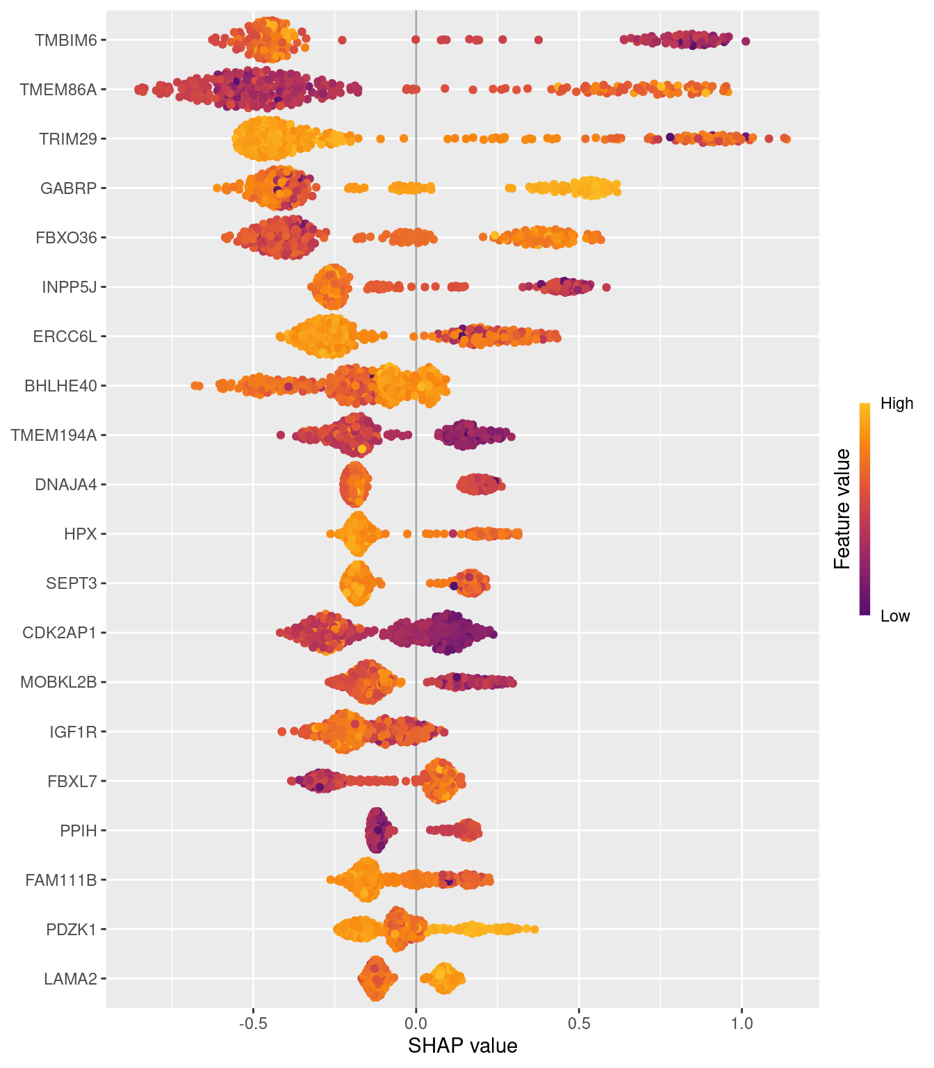
The beeswarm shows the top 20 genes by mean |SHAP|. Each dot is one sample, coloured by expression level (red = high, blue = low). The SHAP values here are aggregated across all four PAM50 classes by treeshap into a single combined importance score per gene. Genes with consistently large |SHAP| values are the strongest overall discriminators across all class boundaries.
XGBoost SHAP vs RF Gini importance
treeshap computes SHAP values for multiclass Random Forest by propagating contributions through each tree, but for this version of the package the RF SHAP matrix is returned mostly as NA (features absent from a given tree’s path are unresolvable for the combined multiclass output). After zero-filling those NAs the RF SHAP importance is flat and uninformative. We therefore compare XGBoost SHAP directly against RF Gini importance — both are legitimate global importance measures, and the comparison remains meaningful.
p_xgb <- sv_importance(sv_xgb, kind = "bar", max_display = 20) +
           ggplot2::ggtitle("XGBoost — mean |SHAP|")

gini_df <- data.frame(
  Feature    = rownames(rf_model$finalModel$importance),
  Importance = rf_model$finalModel$importance[, "MeanDecreaseGini"]
) |>
  dplyr::arrange(dplyr::desc(Importance)) |>
  head(20)

p_rf <- ggplot2::ggplot(gini_df,
          ggplot2::aes(x = Importance, y = reorder(Feature, Importance))) +
          ggplot2::geom_col(fill = "#4472C4") +
          ggplot2::labs(x = "Mean decrease Gini", y = NULL,
                        title = "Random Forest — Gini importance") +
          ggplot2::theme_bw()

p_xgb + p_rf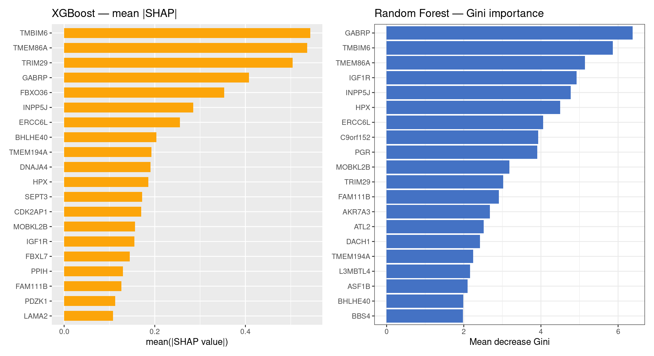
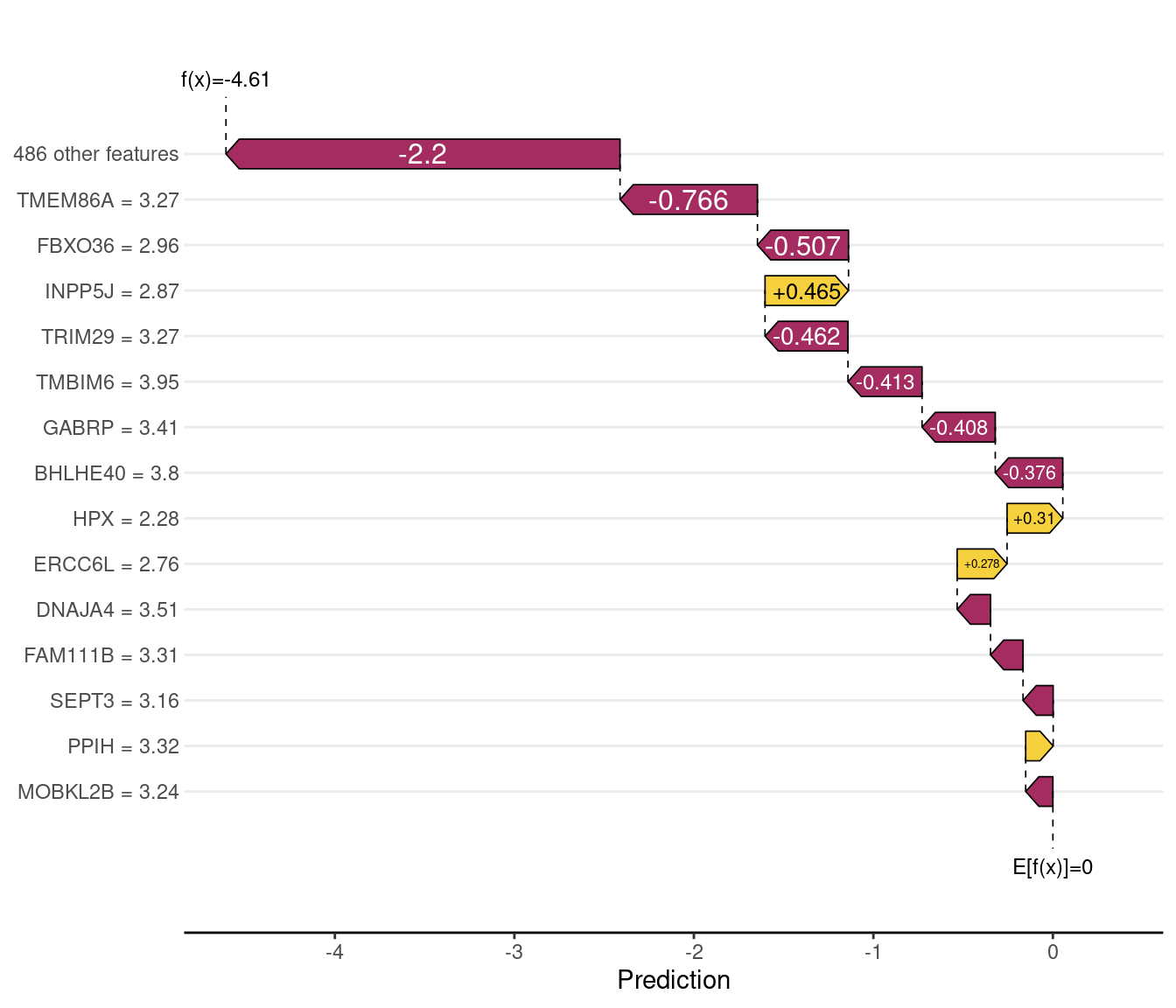
Waterfall plots — individual sample explanations
A waterfall plot decomposes one prediction into its feature contributions. The baseline (leftmost bar) is the model’s average prediction across training data; each subsequent bar adds the SHAP contribution of one gene. The final value is the model’s output for that sample. Comparing a correctly classified and a misclassified sample reveals which features led the model astray.
# Identify one correctly and one incorrectly classified sample using 5-fold CV probabilities.
# xgb_probs is the n×4 held-out probability matrix from xgb_cv_probs().
pred_class  <- colnames(xgb_probs)[apply(xgb_probs, 1, which.max)]
correct_idx <- which(pred_class == as.character(y))[1]
wrong_idx   <- which(pred_class != as.character(y))
wrong_idx   <- if (length(wrong_idx) > 0) wrong_idx[1] else which.min(apply(xgb_probs, 1, max))

cat("Correctly classified — index:", correct_idx,
    "| true:", as.character(y)[correct_idx],
    "| predicted:", pred_class[correct_idx], "\n")
Correctly classified — index: 1 | true: Basal | predicted: Basal cat("Misclassified — index:", wrong_idx,
"| true:", as.character(y)[wrong_idx],
"| predicted:", pred_class[wrong_idx], "\n")Misclassified — index: 8 | true: Basal | predicted: LumA 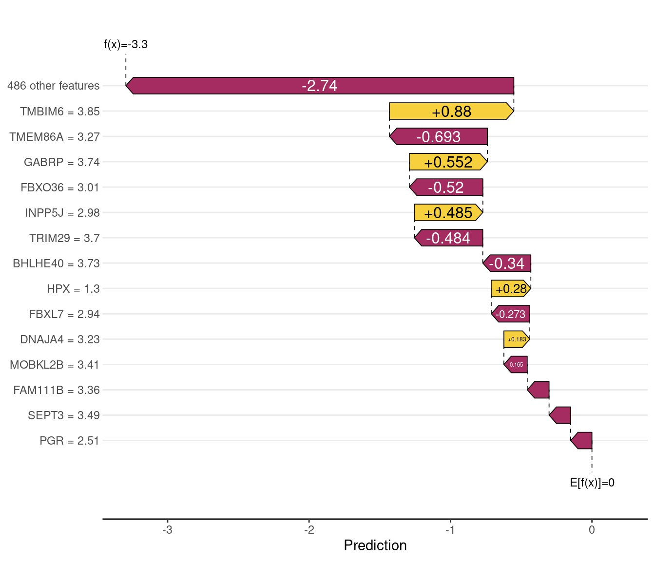
Three-way importance comparison: Gini / Gain / SHAP
Spearman rank correlations (top 20 by SHAP-XGBoost):
  Gini vs SHAP-XGB: 0.683
Gain vs SHAP-XGB: 0.86 | Gene | SHAP-XGB rank | Gain rank | Gini rank | |
|---|---|---|---|---|
| TMBIM6 | TMBIM6 | 1 | 1 | 2 |
| TMEM86A | TMEM86A | 2 | 2 | 3 |
| TRIM29 | TRIM29 | 3 | 5 | 11 |
| GABRP | GABRP | 4 | 4 | 1 |
| FBXO36 | FBXO36 | 5 | 9 | 23 |
| ERCC6L | ERCC6L | 6 | 3 | 7 |
| INPP5J | INPP5J | 7 | 6 | 5 |
| BHLHE40 | BHLHE40 | 8 | 7 | 19 |
| HPX | HPX | 9 | 10 | 6 |
| CDK2AP1 | CDK2AP1 | 10 | 15 | 21 |
| DNAJA4 | DNAJA4 | 11 | 48 | 136 |
| TMEM194A | TMEM194A | 12 | 14 | 16 |
| FAM111B | FAM111B | 13 | 8 | 12 |
| MOBKL2B | MOBKL2B | 14 | 12 | 10 |
| IGF1R | IGF1R | 15 | 11 | 4 |
| SEPT3 | SEPT3 | 16 | 24 | 79 |
| ERI2 | ERI2 | 17 | 46 | 196 |
| FBXL7 | FBXL7 | 18 | 33 | 41 |
| EIF3D | EIF3D | 19 | 56 | 194 |
| PDZK1 | PDZK1 | 20 | 18 | 26 |
Interpreting the three-way table: Genes near rank 1 across all four columns (SHAP-XGB, SHAP-RF, Gain, Gini) are the most algorithm-agnostic PAM50 markers — the signal is strong enough that every metric and every model finds them. Genes with high SHAP rank but low Gini/gain rank (or vice versa) are worth investigating: they may reflect features that are globally used many times in shallow splits (high Gini/gain) but whose per-sample contributions average out, or conversely, features that provide decisive contributions in a subset of samples even if rarely used overall.
Expected biological check: ESR1, GATA3, FOXA1 (LumA markers), ERBB2, GRB7 (HER2 markers), KRT5, KRT14 (Basal markers), and MKI67, TOP2A (proliferation) should appear in the top 10 of at least one SHAP column. If they do not, check that xgb_final and rf_model are the BRCA models (not the simulated-data models).
Class Imbalance
Real genomics datasets often have severe class imbalance (e.g., 95% controls, 5% cases). Below we show how to enable SMOTE-based correction within the caret framework.
# Requires the 'themis' package: install.packages("themis")
library(themis)

ctrl_smote <- trainControl(
  method          = "cv",
  number          = 5,
  classProbs      = TRUE,
  summaryFunction = twoClassSummary,
  sampling        = "smote"   # oversample minority class
)

# Then use ctrl_smote in place of ctrl_loocv in any train() call above
For further discussion of class imbalance strategies, see Section 0.9 and the exercises below.
Exercises
Signal-to-noise ratio — Retrain the Random Forest varying the number of signal genes (top variable) mixed with 450 noise genes: try 10, 25, 100, and 500 signal genes. Plot AUC vs. signal gene count. At what point does performance collapse? What does this tell you about feature selection in high-dimensional genomics data?
Binary subproblem — Instead of 4-class classification, train a binary RF on just two subtypes: the most similar pair (LumA vs LumB — both ER+, differ in proliferation) and the most different pair (Basal vs LumA — triple-negative vs strongly ER+). Does AUC improve for the easy pair and drop for the hard pair? What does this tell you about the difficulty of each pairwise boundary?
Permutation test — Shuffle the subtype labels randomly and retrain the RF. What multiclass AUC do you get? What does this baseline tell you about the significance of your original result?
Biological interpretation — Look up the top 5 RF importance genes in GeneCards or NCBI Gene. Are they known PAM50 subtype markers (e.g. ESR1, ERBB2, KRT5, MKI67)? Do their expression directions match known biology (e.g. ESR1 high in LumA, low in Basal)?
Sample size effect — Retrain all three classifiers using only 25, 50, and 75 samples per subtype. Plot multiclass AUC vs n. At what n does XGBoost start to match RF? Does the crossover point match the n > ~50 per class rule of thumb?
Starter code:
SHAP for a binary subproblem — Repeat the SHAP analysis on a binary classifier trained on just LumA vs LumB (the hardest pairwise boundary from Exercise 2). Do the same genes appear in the SHAP top 20 as in the 4-class analysis? What does this reveal about subtype-specific markers (LumA/LumB-specific) vs general discriminators (used in all pairwise comparisons)? Note that for a binary model, the shapviz object will be a single rather than an , so is not needed — use directly.
Session Info
R version 4.5.1 (2025-06-13)
Platform: x86_64-pc-linux-gnu
Running under: Debian GNU/Linux 11 (bullseye)

Matrix products: default
BLAS:   /usr/lib/x86_64-linux-gnu/blas/libblas.so.3.9.0
LAPACK: /usr/lib/x86_64-linux-gnu/lapack/liblapack.so.3.9.0  LAPACK version 3.9.0

locale:
 [1] LC_CTYPE=en_US.UTF-8       LC_NUMERIC=C               LC_TIME=en_US.UTF-8        LC_COLLATE=en_US.UTF-8     LC_MONETARY=en_US.UTF-8    LC_MESSAGES=en_US.UTF-8    LC_PAPER=en_US.UTF-8       LC_NAME=C
 [9] LC_ADDRESS=C               LC_TELEPHONE=C             LC_MEASUREMENT=en_US.UTF-8 LC_IDENTIFICATION=C

time zone: America/Los_Angeles
tzcode source: system (glibc)

attached base packages:
[1] stats4    stats     graphics  grDevices utils     datasets  methods   base

other attached packages:
 [1] curatedTCGAData_1.32.1      MultiAssayExperiment_1.36.2 SummarizedExperiment_1.40.0 Biobase_2.70.0              GenomicRanges_1.62.1        Seqinfo_1.0.0               IRanges_2.44.0
 [8] S4Vectors_0.48.1            BiocGenerics_0.56.0         generics_0.1.4              MatrixGenerics_1.22.0       matrixStats_1.5.0           caret_7.0-1                 lattice_0.22-7
[15] patchwork_1.3.2             shapviz_0.10.3              treeshap_0.4.0              ggrepel_0.9.8               pheatmap_1.0.13             pROC_1.19.0.1               e1071_1.7-17
[22] xgboost_3.2.1.1             randomForest_4.7-1.2        lubridate_1.9.5             forcats_1.0.1               stringr_1.6.0               dplyr_1.2.1                 purrr_1.2.2
[29] readr_2.2.0                 tidyr_1.3.2                 tibble_3.3.1                ggplot2_4.0.2               tidyverse_2.0.0

loaded via a namespace (and not attached):
  [1] RColorBrewer_1.1-3   jsonlite_2.0.0       magrittr_2.0.5       farver_2.1.2         rmarkdown_2.31       vctrs_0.7.3          ROCR_1.0-12          shades_1.4.0         memoise_2.0.1        htmltools_0.5.9
 [11] S4Arrays_1.10.1      BiocBaseUtils_1.12.0 AnnotationHub_4.0.0  curl_7.0.0           SparseArray_1.10.10  parallelly_1.47.0    htmlwidgets_1.6.4    plyr_1.8.9           httr2_1.2.2          cachem_1.1.0
 [21] ggfittext_0.10.3     lifecycle_1.0.5      iterators_1.0.14     pkgconfig_2.0.3      Matrix_1.7-5         R6_2.6.1             fastmap_1.2.0        future_1.70.0        digest_0.6.39        AnnotationDbi_1.72.0
 [31] ExperimentHub_3.0.0  RSQLite_2.4.6        filelock_1.0.3       labeling_0.4.3       timechange_0.4.0     httr_1.4.8           abind_1.4-8          compiler_4.5.1       proxy_0.4-29         bit64_4.6.0-1
 [41] withr_3.0.2          S7_0.2.1-1           DBI_1.3.0            MASS_7.3-65          lava_1.9.0           rappdirs_0.3.4       DelayedArray_0.36.1  ModelMetrics_1.2.2.2 tools_4.5.1          otel_0.2.0
 [51] future.apply_1.20.2  nnet_7.3-20          glue_1.8.1           nlme_3.1-168         grid_4.5.1           reshape2_1.4.5       gggenes_0.6.0        recipes_1.3.2        gtable_0.3.6         tzdb_0.5.0
 [61] class_7.3-23         data.table_1.18.2.1  hms_1.1.4            XVector_0.50.0       BiocVersion_3.22.0   foreach_1.5.2        pillar_1.11.1        splines_4.5.1        BiocFileCache_3.0.0  survival_3.8-3
 [71] bit_4.6.0            tidyselect_1.2.1     Biostrings_2.78.0    knitr_1.51           xfun_0.57            hardhat_1.4.3        timeDate_4052.112    stringi_1.8.7        yaml_2.3.12          MLmetrics_1.1.3
 [81] evaluate_1.0.5       codetools_0.2-20     kernlab_0.9-33       BiocManager_1.30.27  cli_3.6.6            rpart_4.1.24         dichromat_2.0-0.1    Rcpp_1.1.1-1         globals_0.19.1       dbplyr_2.5.2
 [91] png_0.1-9            parallel_4.5.1       gower_1.0.2          blob_1.3.0           listenv_0.10.1       viridisLite_0.4.3    ipred_0.9-15         scales_1.4.0         prodlim_2026.03.11   crayon_1.5.3
[101] rlang_1.2.0 KEGGREST_1.50.0 References
Chen, Tianqi, and Carlos Guestrin. 2016. “XGBoost: A Scalable Tree Boosting System.” arXiv [Cs.LG], March. https://doi.org/10.48550/arXiv.1603.02754.
Díaz-Uriarte, Ramón, and Sara Alvarez de Andrés. 2006. “Gene selection and classification of microarray data using random forest.” BMC Bioinformatics 7 (1): 3. https://doi.org/10.1186/1471-2105-7-3.
Lundberg, Scott M, Gabriel Erion, Hugh Chen, Alex DeGrave, Jordan M Prutkin, Bala Nair, Ronit Katz, Jonathan Himmelfarb, Nisha Bansal, and Su-In Lee. 2020. “From local explanations to global understanding with explainable AI for trees.” Nat. Mach. Intell. 2 (1): 56–67. https://doi.org/10.1038/s42256-019-0138-9.
Qi, Yanjun. 2012. “Random Forest for Bioinformatics.” In Ensemble Machine Learning: Methods and Applications, edited by Cha Zhang and Yunqian Ma, 307–23. New York, NY: Springer New York. https://doi.org/10.1007/978-1-4419-9326-7_11.