Cluster Analysis in R

Author

First/last name (first.last@ucr.edu)

Published

March 28, 2026

Introduction

What is Clustering?
- Clustering is the classification of data objects into similarity groups (clusters) according to a defined distance measure.
- It is used in many fields, such as machine learning, data mining, pattern recognition, image analysis, genomics, systems biology, etc.
- Machine learning typically regards data clustering as a form of unsupervised learning.
Why Clustering and Data Mining in R?}
- Efficient data structures and functions for clustering
- Reproducible and programmable
- Comprehensive set of clustering and machine learning libraries
- Integration with many other data analysis tools
Useful Links

Data Preprocessing

Data Transformations

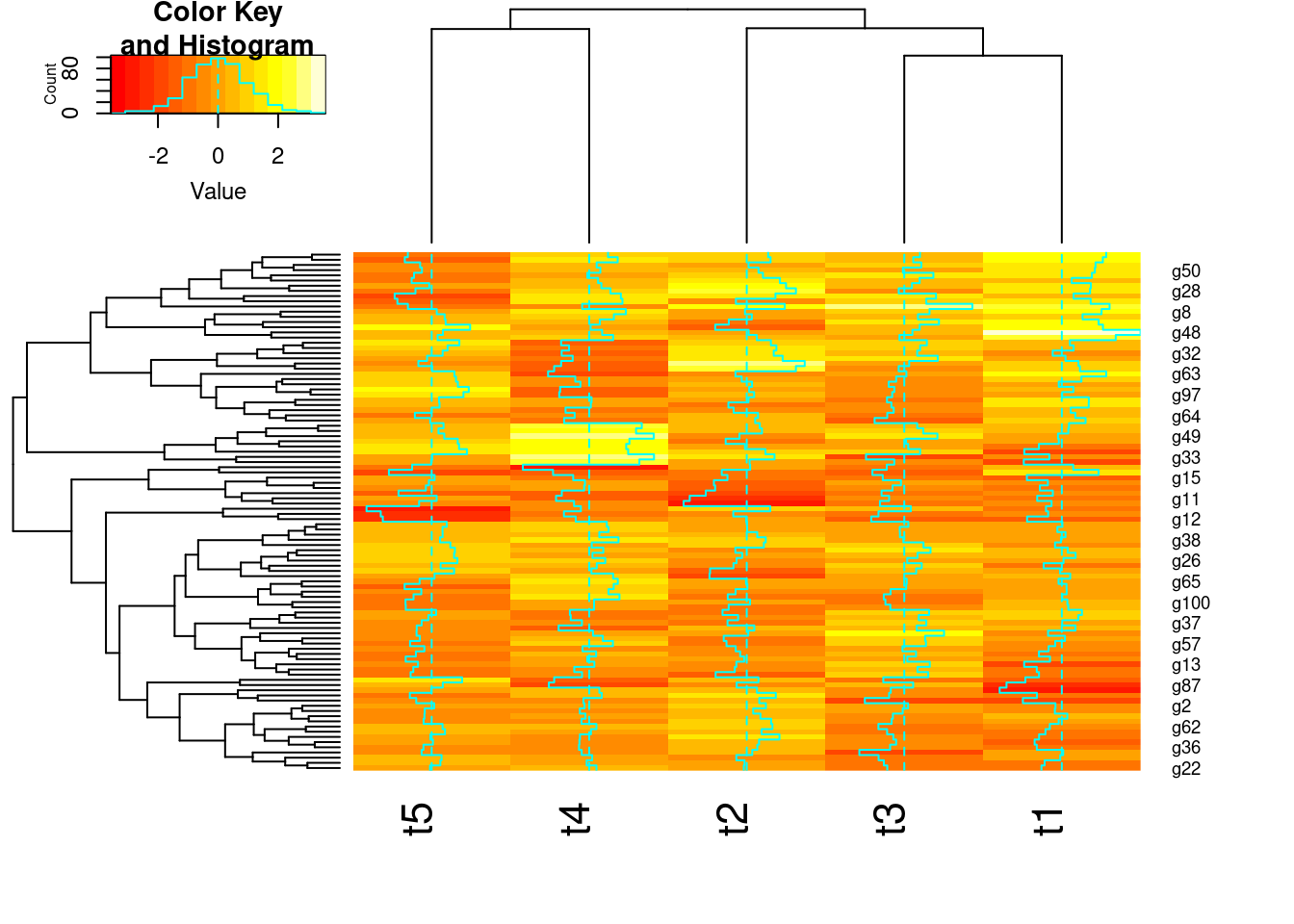
Choice depends on data set!

Center and standardize
1. Center: subtract from each value the mean of the corresponding vector
2. Standardize: devide by standard deviation
  - Result: Mean = 0 and STDEV = 1
Center and scale with the scale() function
1. Center: subtract from each value the mean of the corresponding vector
2. Scale: divide centered vector by their root mean square (rms):
  - Result: Mean = 0 and STDEV = 1 \[ x_{rms} = \sqrt[]{\frac{1}{n-1}\sum_{i=1}^{n}{x_{i}{^2}}} \]
Log transformation
Rank transformation: replace measured values by ranks
No transformation

Distance Methods

List of most common ones!

Euclidean distance for two profiles X and Y: \[ d(X,Y) = \sqrt[]{ \sum_{i=1}^{n}{(x_{i}-y_{i})^2} }\]
- Disadvantages: not scale invariant, not for negative correlations
Maximum, Manhattan, Canberra, binary, Minowski, …
Correlation-based distance: 1-r
- Pearson correlation coefficient (PCC): \[r = \frac{n\sum_{i=1}^{n}{x_{i}y_{i}} - \sum_{i=1}^{n}{x_{i}} \sum_{i=1}^{n}{y_{i}}}{ \sqrt[]{(\sum_{i=1}^{n}{x_{i}^2} - (\sum_{i=1}^{n}{x_{i})^2}) (\sum_{i=1}^{n}{y_{i}^2} - (\sum_{i=1}^{n}{y_{i})^2})} }\] Disadvantage: outlier sensitive
- Spearman correlation coefficient (SCC): Same calculation as PCC but with ranked values!

There are many more distance measures

If the distances among items are quantifiable, then clustering is possible.
Choose the most accurate and meaningful distance measure for a given field of application.
If uncertain then choose several distance measures and compare the results.

Cluster Linkage

Clustering Algorithms

Hierarchical Clustering

Overview of algorithm

Identify clusters (items) with closest distance
Join them to new clusters
Compute distance between clusters (items)
Return to step 1

Hierarchical clustering: agglomerative Approach

Hierarchical Clustering with Heatmap

A heatmap is a color coded table. To visually identify patterns, the rows and columns of a heatmap are often sorted by hierarchical clustering trees.
In case of gene expression data, the row tree usually represents the genes, the column tree the treatments and the colors in the heat table represent the intensities or ratios of the underlying gene expression data set.

Hierarchical Clustering Approaches

Agglomerative approach (bottom-up)
- R functions: hclust() and agnes()
Divisive approach (top-down)
- R function: diana()

Tree Cutting to Obtain Discrete Clusters

Node height in tree
Number of clusters
Search tree nodes by distance cutoff

Examples

Required packages

The code sections in this tutorial make use of the following R/Bioc packages: c("ggplot2", "gplots", "pheatmap", "RColorBrewer", "ape", "ComplexHeatmap", "scatterplot3d"). If they are not available on a system, then they need to be installed with BiocManager::install() first.

Using `hclust` and `heatmap.2`

Note, with large data sets consider using flashClust which is a fast implementation of hierarchical clustering.

library(gplots) 
y <- matrix(rnorm(500), 100, 5, dimnames=list(paste("g", 1:100, sep=""), paste("t", 1:5, sep=""))) 
heatmap.2(y) # Shortcut to final result

Stepwise Approach with Tree Cutting

## Row- and column-wise clustering 
hr <- hclust(as.dist(1-cor(t(y), method="pearson")), method="complete")
hc <- hclust(as.dist(1-cor(y, method="spearman")), method="complete") 
## Tree cutting
mycl <- cutree(hr, h=max(hr$height)/1.5); mycolhc <- rainbow(length(unique(mycl)), start=0.1, end=0.9); mycolhc <- mycolhc[as.vector(mycl)] 
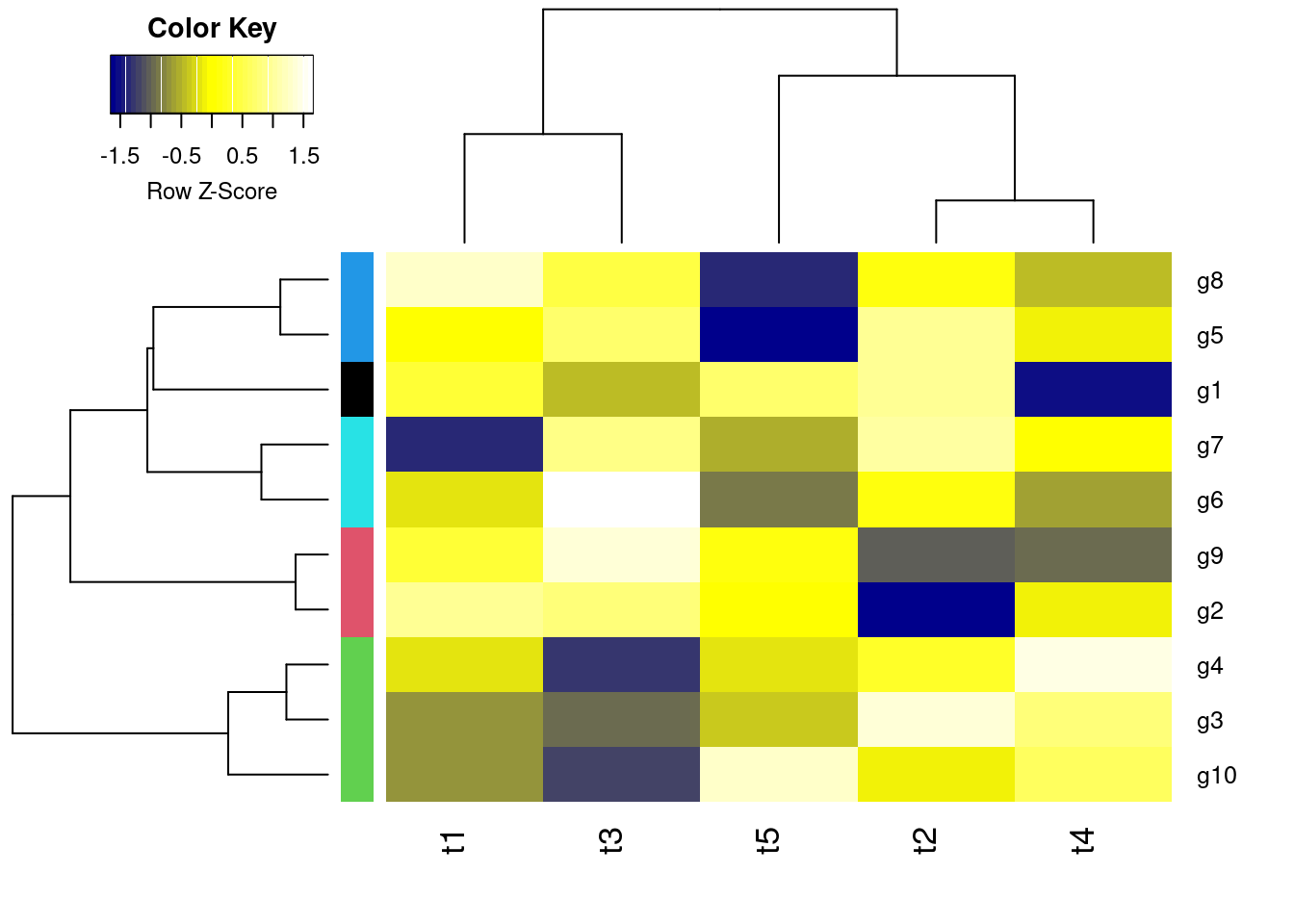
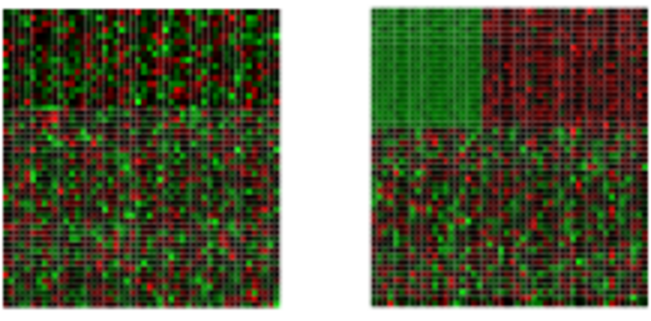
## Plot heatmap 
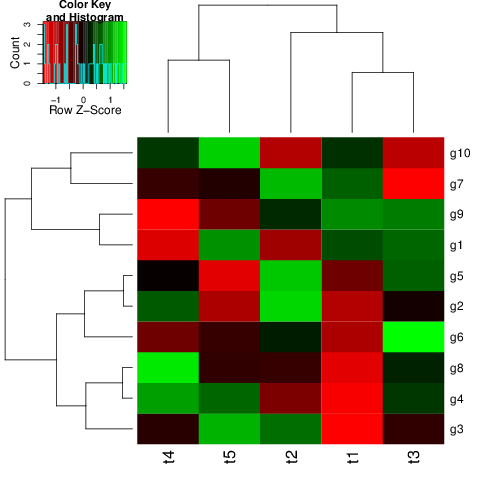
mycol <- colorpanel(40, "darkblue", "yellow", "white") # or try redgreen(75)
heatmap.2(y, Rowv=as.dendrogram(hr), Colv=as.dendrogram(hc), col=mycol, scale="row", density.info="none", trace="none", RowSideColors=mycolhc)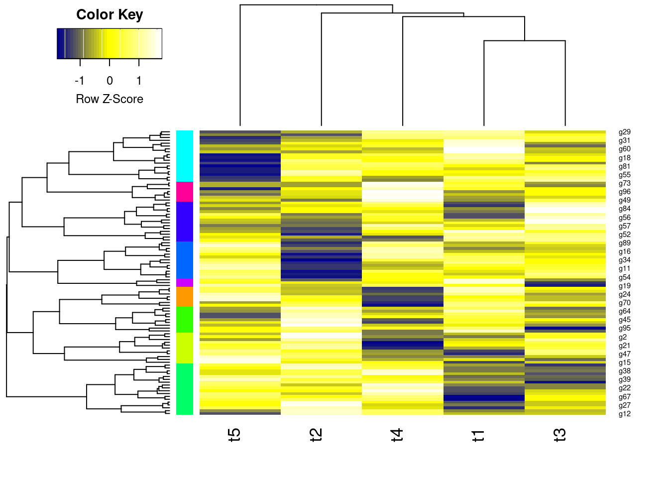

K-Means Clustering

Overview of algorithm

Choose the number of k clusters
Randomly assign items to the k clusters
Calculate new centroid for each of the k clusters
Calculate the distance of all items to the k centroids
Assign items to closest centroid
Repeat until clusters assignments are stable

Examples

km <- kmeans(t(scale(t(y))), 3)
km$cluster

  g1   g2   g3   g4   g5   g6   g7   g8   g9  g10  g11  g12  g13  g14  g15  g16  g17  g18  g19  g20  g21  g22  g23  g24  g25  g26  g27  g28  g29  g30  g31  g32  g33  g34  g35  g36  g37  g38  g39  g40  g41  g42  g43  g44 
   2    3    1    1    1    1    1    2    1    2    2    3    1    2    1    3    3    2    2    1    1    3    3    2    2    1    3    1    1    3    3    1    3    1    3    3    1    2    2    2    2    1    3    3 
 g45  g46  g47  g48  g49  g50  g51  g52  g53  g54  g55  g56  g57  g58  g59  g60  g61  g62  g63  g64  g65  g66  g67  g68  g69  g70  g71  g72  g73  g74  g75  g76  g77  g78  g79  g80  g81  g82  g83  g84  g85  g86  g87  g88 
   2    2    1    1    1    1    2    2    3    3    2    2    3    2    2    1    1    1    3    2    2    3    1    1    2    2    2    3    2    1    3    3    2    3    2    1    1    3    3    3    1    1    2    3 
 g89  g90  g91  g92  g93  g94  g95  g96  g97  g98  g99 g100 
   2    1    1    2    3    1    1    1    3    2    2    2

Fuzzy C-Means Clustering

In contrast to strict (hard) clustering approaches, fuzzy (soft) clustering methods allow multiple cluster memberships of the clustered items (Hathaway, Bezdek, and Pal 1996).
This is commonly achieved by assigning to each item a weight of belonging to each cluster.
Thus, items at the edge of a cluster, may be in a cluster to a lesser degree than items at the center of a cluster.
Typically, each item has as many coefficients (weights) as there are clusters that sum up for each item to one.

Examples

Fuzzy Clustering with `fanny`

library(cluster) # Loads the cluster library.
fannyy <- fanny(y, k=4, metric = "euclidean", memb.exp = 1.2)
round(fannyy$membership, 2)[1:4,]

   [,1] [,2] [,3] [,4]
g1 0.74 0.05 0.07 0.15
g2 0.03 0.84 0.05 0.08
g3 0.23 0.05 0.59 0.13
g4 0.01 0.01 0.93 0.05

fannyy$clustering # Hard clustering result

  g1   g2   g3   g4   g5   g6   g7   g8   g9  g10  g11  g12  g13  g14  g15  g16  g17  g18  g19  g20  g21  g22  g23  g24  g25  g26  g27  g28  g29  g30  g31  g32  g33  g34  g35  g36  g37  g38  g39  g40  g41  g42  g43  g44 
   1    2    3    3    3    4    4    1    4    4    4    2    3    1    4    4    1    1    4    4    4    1    3    1    1    4    1    3    3    4    1    1    2    4    2    2    3    1    4    1    1    3    1    2 
 g45  g46  g47  g48  g49  g50  g51  g52  g53  g54  g55  g56  g57  g58  g59  g60  g61  g62  g63  g64  g65  g66  g67  g68  g69  g70  g71  g72  g73  g74  g75  g76  g77  g78  g79  g80  g81  g82  g83  g84  g85  g86  g87  g88 
   1    1    3    3    4    4    1    4    2    1    1    1    2    4    4    4    3    4    2    1    4    1    3    3    1    1    1    2    4    4    2    2    4    2    4    4    3    2    2    2    3    4    4    2 
 g89  g90  g91  g92  g93  g94  g95  g96  g97  g98  g99 g100 
   1    3    3    4    2    3    3    3    2    1    1    1

(fannyyMA <- fannyy$membership > 0.20)[1:4,] # Soft clustering result

    [,1]  [,2]  [,3]  [,4]
g1  TRUE FALSE FALSE FALSE
g2 FALSE  TRUE FALSE FALSE
g3  TRUE FALSE  TRUE FALSE
g4 FALSE FALSE  TRUE FALSE

apply(fannyyMA, 1, which)[1:4] # First 4 clusters

$g1
[1] 1

$g2
[1] 2

$g3
[1] 1 3

$g4
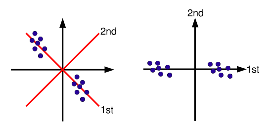
[1] 3

Principal Component Analysis (PCA)

Principal components analysis (PCA) is a data reduction technique that allows to simplify multidimensional data sets to 2 or 3 dimensions for plotting purposes and visual variance analysis.

Basic Steps

Center (and standardize) data
First principal component axis
- Across centroid of data cloud
- Distance of each point to that line is minimized, so that it crosses the maximum variation of the data cloud
Second principal component axis
- Orthogonal to first principal component
- Along maximum variation in the data
First PCA axis becomes x-axis and second PCA axis y-axis
Continue process until the necessary number of principal components is obtained

Example

pca <- prcomp(y, scale=T)
summary(pca) # Prints variance summary for all principal components

Importance of components:
                          PC1    PC2    PC3    PC4    PC5
Standard deviation     1.1715 1.0232 0.9814 0.9439 0.8524
Proportion of Variance 0.2745 0.2094 0.1926 0.1782 0.1453
Cumulative Proportion  0.2745 0.4839 0.6765 0.8547 1.0000

plot(pca$x, pch=20, col="blue", type="n") # To plot dots, drop type="n"
text(pca$x, rownames(pca$x), cex=0.8)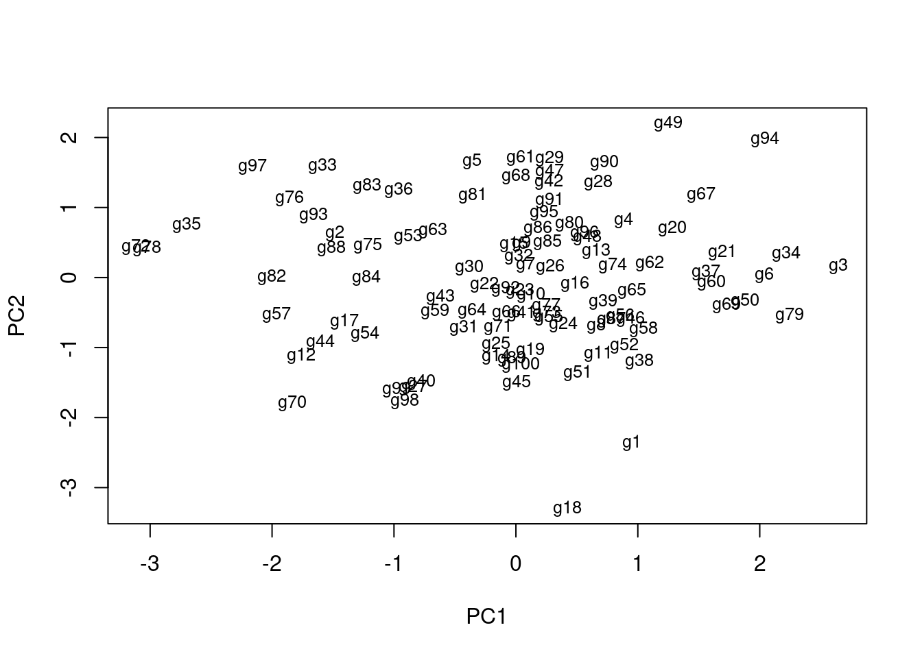

1st and 2nd principal components explain x% of variance in data.

Multidimensional Scaling (MDS)

Alternative dimensionality reduction approach
Represents distances in 2D or 3D space
Starts from distance matrix (PCA uses data points)

Example

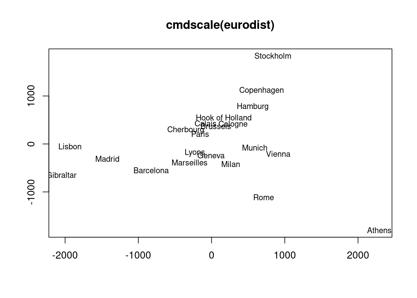
The following example performs MDS analysis with cmdscale on the geographic distances among European cities.

loc <- cmdscale(eurodist) 
plot(loc[,1], -loc[,2], type="n", xlab="", ylab="", main="cmdscale(eurodist)")
text(loc[,1], -loc[,2], rownames(loc), cex=0.8)

Biclustering

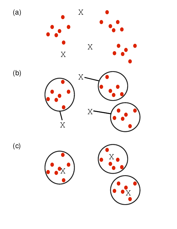
Finds in matrix subgroups of rows and columns which are as similar as possible to each other and as different as possible to the remaining data points.

Similarity Measures for Clusters

Compare the numbers of identical and unique item pairs appearing in cluster sets
Achieved by counting the number of item pairs found in both clustering sets (a) as well as the pairs appearing only in the first (b) or the second (c) set.
With this a similarity coefficient, such as the Jaccard index, can be computed. The latter is defined as the size of the intersect divided by the size of the union of two sample sets: a/(a+b+c).
In case of partitioning results, the Jaccard Index measures how frequently pairs of items are joined together in two clustering data sets and how often pairs are observed only in one set.
Related coefficient are the Rand Index and the Adjusted Rand Index. These indices also consider the number of pairs (d) that are not joined together in any of the clusters in both sets.

Example:

Jaccard index for cluster sets

The following imports the cindex() function and computes the Jaccard Index for two sample cluster results.

source("http://faculty.ucr.edu/~tgirke/Documents/R_BioCond/My_R_Scripts/clusterIndex.R") 
library(cluster); y <- matrix(rnorm(5000), 1000, 5, dimnames=list(paste("g", 1:1000, sep=""), paste("t", 1:5, sep=""))); clarax <- clara(y, 49); clV1 <- clarax$clustering; clarax <- clara(y, 50); clV2 <- clarax$clustering 
ci <- cindex(clV1=clV1, clV2=clV2, self=FALSE, minSZ=1, method="jaccard")
ci[2:3] # Returns Jaccard index and variables used to compute it

$variables
    a     b     c 
11855   873   558 

$Jaccard_Index
[1] 0.8922926

Clustering cluster sets with Jaccard index

The following example shows how one can cluster entire cluster result sets. First, 10 sample cluster results are created with Clara using k-values from 3 to 12. The results are stored as named clustering vectors in a list object. Then a nested sapply loop is used to generate a similarity matrix of Jaccard Indices for the clustering results. After converting the result into a distance matrix, hierarchical clustering is performed with hclust.}

clVlist <- lapply(3:12, function(x) clara(y[1:30, ], k=x)$clustering); names(clVlist) <- paste("k", "=", 3:12)
d <- sapply(names(clVlist), function(x) sapply(names(clVlist), function(y) cindex(clV1=clVlist[[y]], clV2=clVlist[[x]], method="jaccard")[[3]]))
hv <- hclust(as.dist(1-d))
plot(as.dendrogram(hv), edgePar=list(col=3, lwd=4), horiz=T, main="Similarities of 10 Clara Clustering Results for k: 3-12")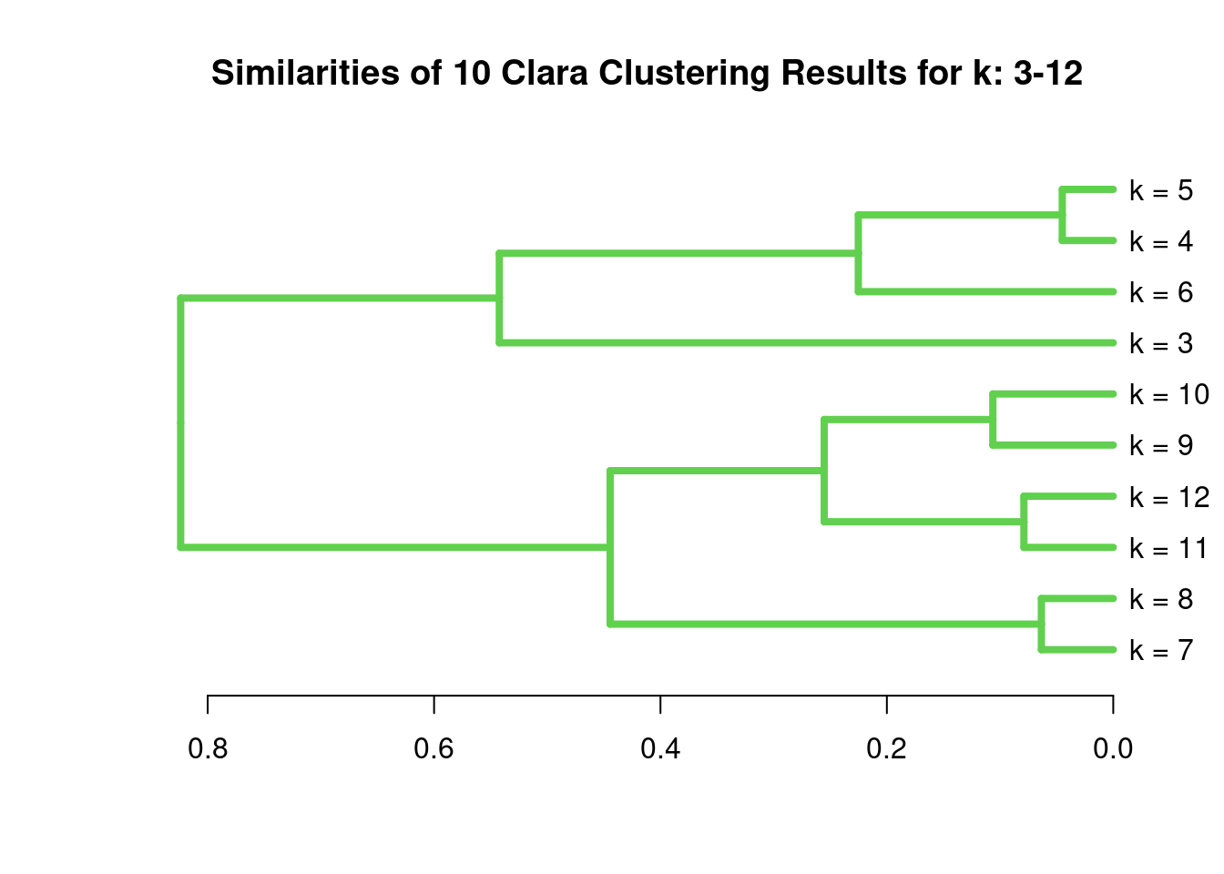

Remember: there are many additional clustering algorithms.
Additional details can be found in the Clustering Section of the R/Bioconductor Manual.

Clustering Exercises

Data Preprocessing

Scaling

## Sample data set
set.seed(1410)
y <- matrix(rnorm(50), 10, 5, dimnames=list(paste("g", 1:10, sep=""), 
            paste("t", 1:5, sep="")))
dim(y)

[1] 10  5

## Scaling
yscaled <- t(scale(t(y))) # Centers and scales y row-wise
apply(yscaled, 1, sd)

 g1  g2  g3  g4  g5  g6  g7  g8  g9 g10 
  1   1   1   1   1   1   1   1   1   1

Distance Matrices

Euclidean distance matrix

dist(y[1:4,], method = "euclidean")

         g1       g2       g3
g2 4.793697                  
g3 4.932658 6.354978         
g4 4.033789 4.788508 1.671968

Correlation-based distance matrix

Correlation matrix

c <- cor(t(y), method="pearson") 
as.matrix(c)[1:4,1:4]

            g1         g2          g3         g4
g1  1.00000000 -0.2965885 -0.00206139 -0.4042011
g2 -0.29658847  1.0000000 -0.91661118 -0.4512912
g3 -0.00206139 -0.9166112  1.00000000  0.7435892
g4 -0.40420112 -0.4512912  0.74358925  1.0000000

Correlation-based distance matrix

d <- as.dist(1-c)
as.matrix(d)[1:4,1:4]

         g1       g2        g3        g4
g1 0.000000 1.296588 1.0020614 1.4042011
g2 1.296588 0.000000 1.9166112 1.4512912
g3 1.002061 1.916611 0.0000000 0.2564108
g4 1.404201 1.451291 0.2564108 0.0000000

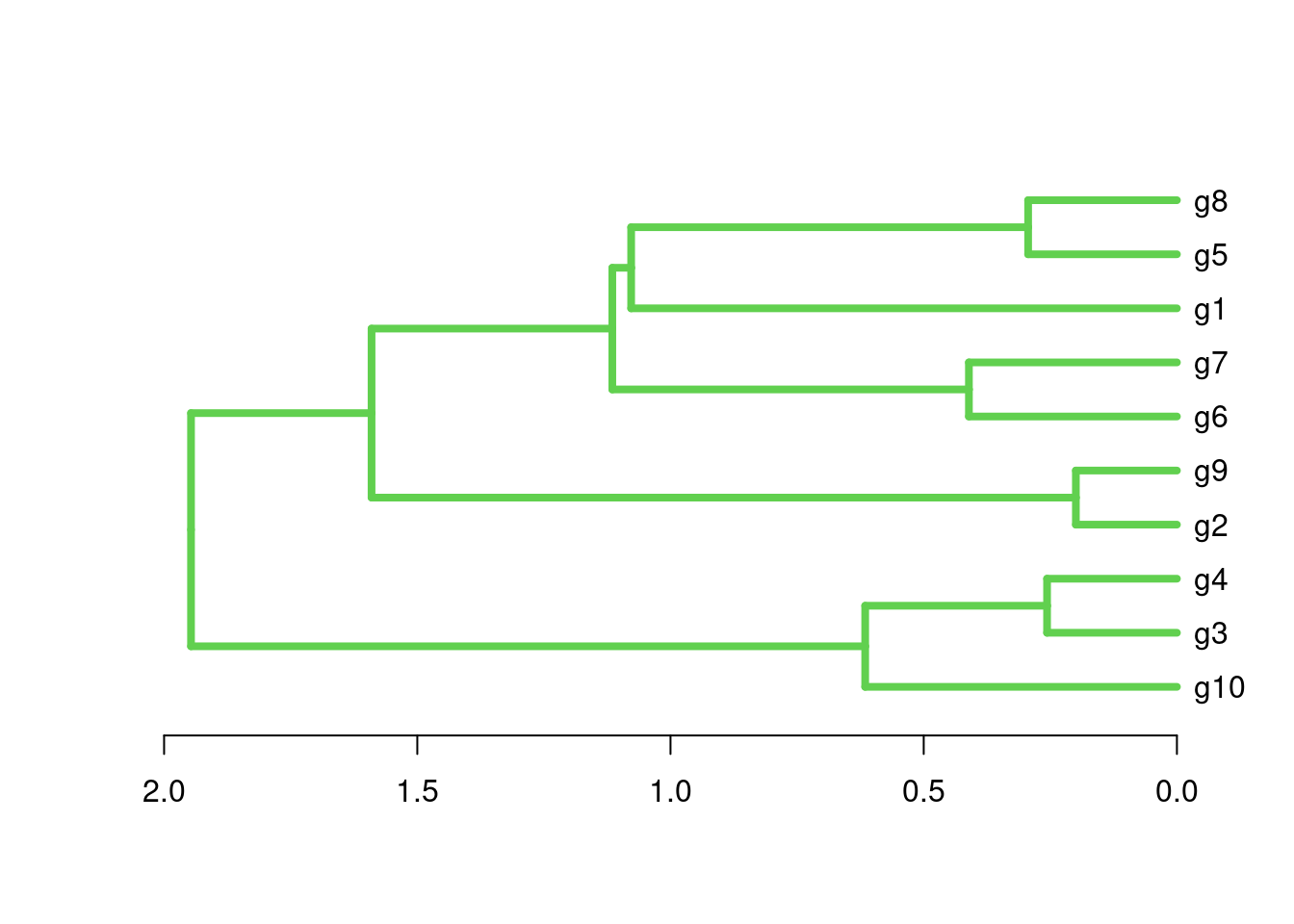
Hierarchical Clustering with `hclust`

Hierarchical clustering with complete linkage and basic tree plotting

hr <- hclust(d, method = "complete", members=NULL)
names(hr)

[1] "merge"       "height"      "order"       "labels"      "method"      "call"        "dist.method"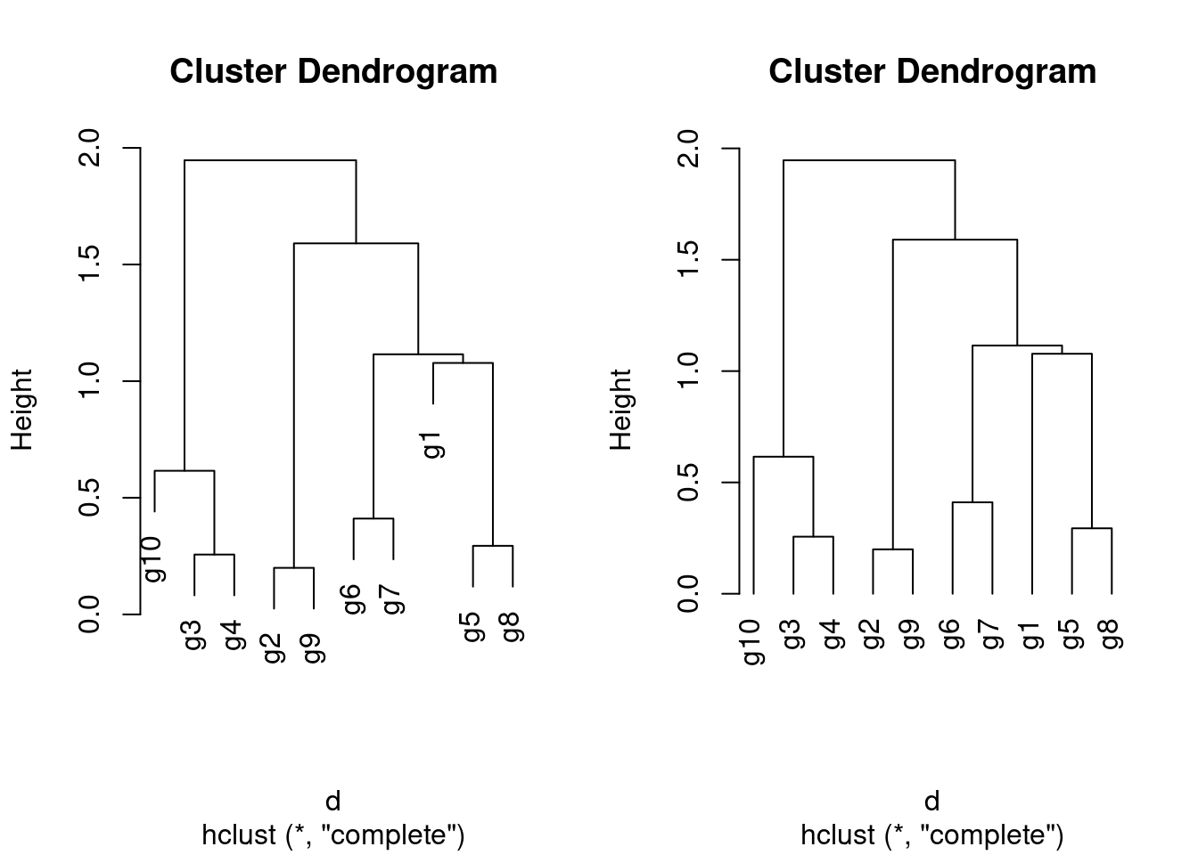

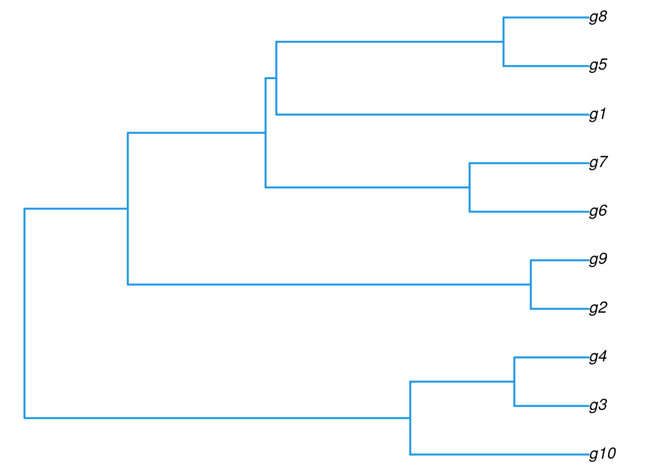
par(mfrow = c(1, 2)); plot(hr, hang = 0.1); plot(hr, hang = -1)

Tree plotting I

plot(as.dendrogram(hr), edgePar=list(col=3, lwd=4), horiz=T)

Tree plotting II

The ape library provides more advanced features for tree plotting

library(ape) 
plot.phylo(as.phylo(hr), type="p", edge.col=4, edge.width=2, 
           show.node.label=TRUE, no.margin=TRUE)

Tree Cutting

Accessing information in hclust objects

hr


Call:
hclust(d = d, method = "complete", members = NULL)

Cluster method   : complete 
Number of objects: 10

## Print row labels in the order they appear in the tree
hr$labels[hr$order]

 [1] "g10" "g3"  "g4"  "g2"  "g9"  "g6"  "g7"  "g1"  "g5"  "g8"

Tree cutting with cutree

mycl <- cutree(hr, h=max(hr$height)/2)
mycl[hr$labels[hr$order]]

g10  g3  g4  g2  g9  g6  g7  g1  g5  g8 
  3   3   3   2   2   5   5   1   4   4

Heatmaps

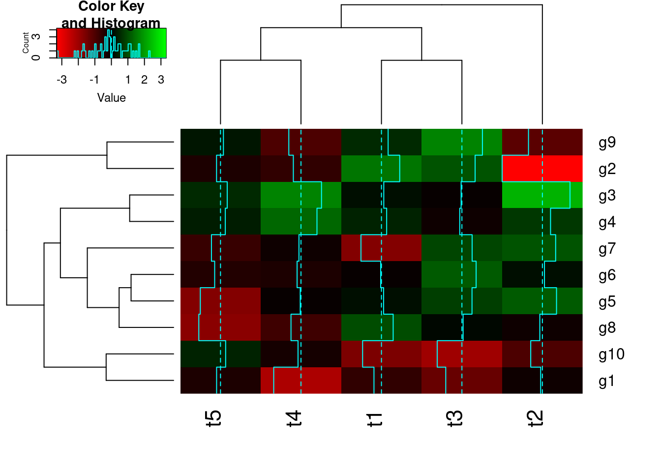
With `heatmap.2`

All in one step: clustering and heatmap plotting

library(gplots)
heatmap.2(y, col=redgreen(75))

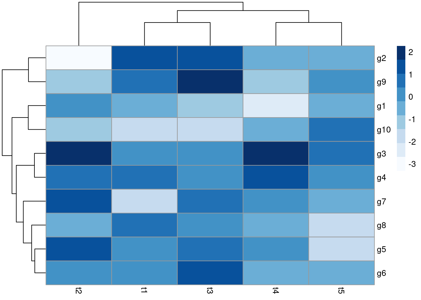
With `pheatmap`

All in one step: clustering and heatmap plotting

library(pheatmap); library("RColorBrewer")
pheatmap(y, color=brewer.pal(9,"Blues"))

Customizing heatmaps

Customizes row and column clustering and shows tree cutting result in row color bar. Additional color schemes can be found here.

hc <- hclust(as.dist(1-cor(y, method="spearman")), method="complete")
mycol <- colorpanel(40, "darkblue", "yellow", "white")
heatmap.2(y, Rowv=as.dendrogram(hr), Colv=as.dendrogram(hc), col=mycol,
          scale="row", density.info="none", trace="none", 
          RowSideColors=as.character(mycl))

Complex heatmaps

For plotting complex heatmaps, the ComplexHeatmap provides useful functionalities. The following creates a sample heatmap. For additional examples, visit the manual here.

library(ComplexHeatmap)
set.seed(123)
mat = matrix(rnorm(100), 10)
rownames(mat) = paste0("R", 1:10)
colnames(mat) = paste0("C", 1:10)
column_ha = HeatmapAnnotation(foo1 = runif(10), bar1 = anno_barplot(runif(10)))
row_ha = rowAnnotation(foo2 = runif(10), bar2 = anno_barplot(runif(10)))
Heatmap(mat, name = "mat", top_annotation = column_ha, right_annotation = row_ha)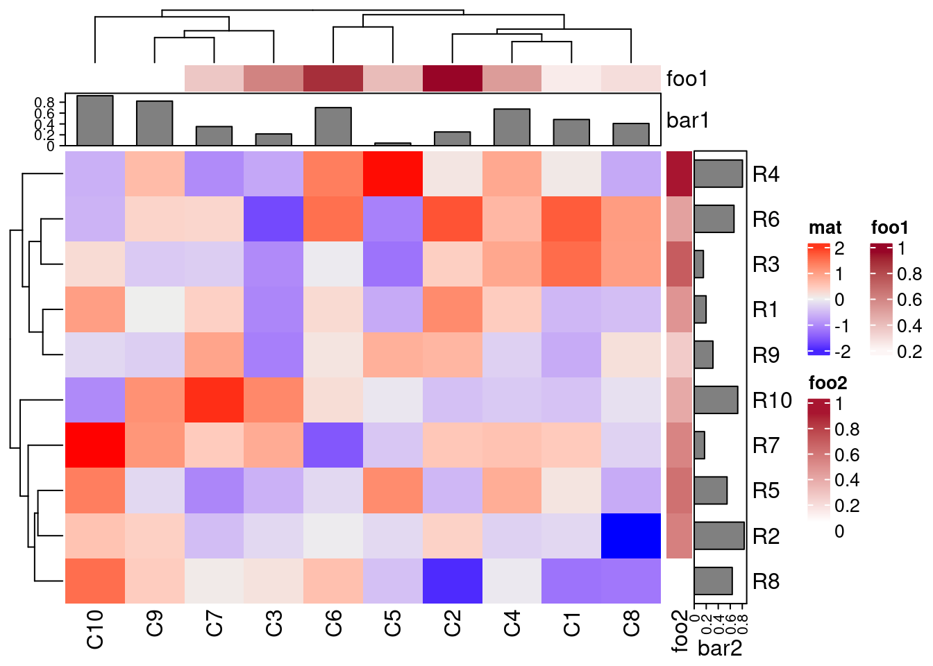

K-Means Clustering with PAM

Runs K-means clustering with PAM (partitioning around medoids) algorithm and shows result in color bar of hierarchical clustering result from before.

library(cluster)
pamy <- pam(d, 4)
(kmcol <- pamy$clustering)

 g1  g2  g3  g4  g5  g6  g7  g8  g9 g10 
  1   2   3   3   4   4   4   4   2   3

heatmap.2(y, Rowv=as.dendrogram(hr), Colv=as.dendrogram(hc), col=mycol,
          scale="row", density.info="none", trace="none", 
          RowSideColors=as.character(kmcol))

K-Means Fuzzy Clustering

Performs k-means fuzzy clustering

library(cluster)
fannyy <- fanny(d, k=4, memb.exp = 1.5)
round(fannyy$membership, 2)[1:4,]

   [,1] [,2] [,3] [,4]
g1 1.00 0.00 0.00 0.00
g2 0.00 0.99 0.00 0.00
g3 0.02 0.01 0.95 0.03
g4 0.00 0.00 0.99 0.01

fannyy$clustering

 g1  g2  g3  g4  g5  g6  g7  g8  g9 g10 
  1   2   3   3   4   4   4   4   2   3

## Returns multiple cluster memberships for coefficient above a certain 
## value (here >0.1)
fannyyMA <- round(fannyy$membership, 2) > 0.10 
apply(fannyyMA, 1, function(x) paste(which(x), collapse="_"))

   g1    g2    g3    g4    g5    g6    g7    g8    g9   g10 
  "1"   "2"   "3"   "3"   "4"   "4"   "4" "2_4"   "2"   "3"

Multidimensional Scaling (MDS)

Performs MDS analysis on the geographic distances between European cities

loc <- cmdscale(eurodist) 
## Plots the MDS results in 2D plot. The minus is required in this example to 
## flip the plotting orientation.
plot(loc[,1], -loc[,2], type="n", xlab="", ylab="", main="cmdscale(eurodist)")
text(loc[,1], -loc[,2], rownames(loc), cex=0.8)

Principal Component Analysis (PCA)

Performs PCA analysis after scaling the data. It returns a list with class prcomp that contains five components: (1) the standard deviations (sdev) of the principal components, (2) the matrix of eigenvectors (rotation), (3) the principal component data (x), (4) the centering (center) and (5) scaling (scale) used.

library(scatterplot3d)
pca <- prcomp(y, scale=TRUE)
names(pca)

[1] "sdev"     "rotation" "center"   "scale"    "x"

summary(pca) # Prints variance summary for all principal components.

Importance of components:
                          PC1    PC2    PC3     PC4    PC5
Standard deviation     1.3611 1.1777 1.0420 0.69264 0.4416
Proportion of Variance 0.3705 0.2774 0.2172 0.09595 0.0390
Cumulative Proportion  0.3705 0.6479 0.8650 0.96100 1.0000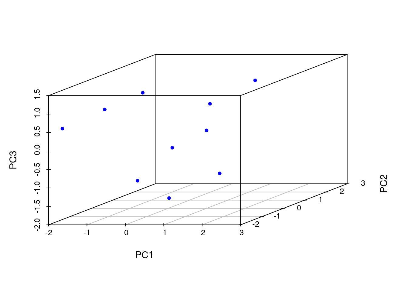

scatterplot3d(pca$x[,1:3], pch=20, color="blue")

Additional Exercises

See here

Version Information

sessionInfo()

R version 4.5.3 (2026-03-11)
Platform: x86_64-pc-linux-gnu
Running under: Debian GNU/Linux 12 (bookworm)

Matrix products: default
BLAS:   /usr/lib/x86_64-linux-gnu/blas/libblas.so.3.11.0 
LAPACK: /usr/lib/x86_64-linux-gnu/lapack/liblapack.so.3.11.0  LAPACK version 3.11.0

locale:
 [1] LC_CTYPE=en_US.UTF-8       LC_NUMERIC=C               LC_TIME=en_US.UTF-8        LC_COLLATE=en_US.UTF-8     LC_MONETARY=en_US.UTF-8    LC_MESSAGES=en_US.UTF-8    LC_PAPER=en_US.UTF-8       LC_NAME=C                 
 [9] LC_ADDRESS=C               LC_TELEPHONE=C             LC_MEASUREMENT=en_US.UTF-8 LC_IDENTIFICATION=C       

time zone: America/Los_Angeles
tzcode source: system (glibc)

attached base packages:
[1] grid      stats     graphics  grDevices utils     datasets  methods   base     

other attached packages:
[1] scatterplot3d_0.3-44  ComplexHeatmap_2.26.1 RColorBrewer_1.1-3    pheatmap_1.0.13       cluster_2.1.8.2       gplots_3.3.0          ape_5.8-1             ggplot2_4.0.2        

loaded via a namespace (and not attached):
 [1] generics_0.1.4      bitops_1.0-9        shape_1.4.6.1       KernSmooth_2.23-26  gtools_3.9.5        lattice_0.22-9      digest_0.6.39       magrittr_2.0.4      caTools_1.18.3      evaluate_1.0.5     
[11] iterators_1.0.14    circlize_0.4.17     fastmap_1.2.0       foreach_1.5.2       doParallel_1.0.17   jsonlite_2.0.0      GlobalOptions_0.1.3 scales_1.4.0        codetools_0.2-20    cli_3.6.5          
[21] rlang_1.1.7         crayon_1.5.3        withr_3.0.2         yaml_2.3.12         otel_0.2.0          tools_4.5.3         parallel_4.5.3      dplyr_1.2.0         colorspace_2.1-2    BiocGenerics_0.56.0
[31] GetoptLong_1.1.0    vctrs_0.7.1         R6_2.6.1            png_0.1-8           magick_2.9.0        stats4_4.5.3        matrixStats_1.5.0   lifecycle_1.0.5     S4Vectors_0.48.0    IRanges_2.44.0     
[41] htmlwidgets_1.6.4   clue_0.3-68         pkgconfig_2.0.3     pillar_1.11.1       gtable_0.3.6        glue_1.8.0          Rcpp_1.1.1          xfun_0.56           tibble_3.3.1        tidyselect_1.2.1   
[51] knitr_1.51          dichromat_2.0-0.1   rjson_0.2.23        farver_2.1.2        htmltools_0.5.9     nlme_3.1-168        rmarkdown_2.30      Cairo_1.7-0         compiler_4.5.3      S7_0.2.1

References

Hathaway, R J, J C Bezdek, and N R Pal. 1996. “Sequential Competitive Learning and the Fuzzy c-Means Clustering Algorithms.” Neural Netw. 9 (5): 787–96. http://www.hubmed.org/display.cgi?uids=12662563.

Introduction

Data Preprocessing

Data Transformations

Distance Methods

Cluster Linkage

Clustering Algorithms

Hierarchical Clustering

Overview of algorithm

Hierarchical clustering: agglomerative Approach

Hierarchical Clustering with Heatmap

Hierarchical Clustering Approaches

Tree Cutting to Obtain Discrete Clusters

Examples

Required packages

Using hclust and heatmap.2

Stepwise Approach with Tree Cutting

K-Means Clustering

Overview of algorithm

Examples

Fuzzy C-Means Clustering

Examples

Fuzzy Clustering with fanny

Principal Component Analysis (PCA)

Basic Steps

Example

Multidimensional Scaling (MDS)

Example

Biclustering

Similarity Measures for Clusters

Example:

Jaccard index for cluster sets

Clustering cluster sets with Jaccard index

Clustering Exercises

Data Preprocessing

Scaling

Distance Matrices

Euclidean distance matrix

Correlation-based distance matrix

Hierarchical Clustering with hclust

Tree plotting I

Tree plotting II

Tree Cutting

Heatmaps

With heatmap.2

With pheatmap

Customizing heatmaps

Complex heatmaps

K-Means Clustering with PAM

K-Means Fuzzy Clustering

Multidimensional Scaling (MDS)

Principal Component Analysis (PCA)

Additional Exercises

Version Information

References

Using `hclust` and `heatmap.2`

Fuzzy Clustering with `fanny`

Hierarchical Clustering with `hclust`

With `heatmap.2`

With `pheatmap`