Quarto & R Markdown Tutorial
Overview
Quarto and R Markdown are literate programming environments that combine plain-text narrative with embedded code. When a document is rendered, the code is executed and its output (tables, figures and equations) is rendered together with the narrative text into a polished HTML, PDF, or Word file. This approach has several important benefits for scientific work:
- Reproducibility: results are regenerated automatically whenever the underlying code or data changes, eliminating manual editing errors between analysis and report.
- Transparency: readers can inspect the exact code that produced every result.
- Collaboration: plain-text source files work naturally with version-control systems such as Git, making it straightforward to track changes and merge contributions.
- Versatility: the same source file can produce a research analysis report, a journal article, a website, or a slide deck with minimal changes.
Quarto (.qmd files) is the current recommended environment and is used for all GEN242 course projects. It is the direct successor to R Markdown (.Rmd files) and is covered here first and in greater depth. R Markdown remains important because it is used extensively in the Bioconductor ecosystem (most package vignettes are written in R Markdown) and in the broader R community; it is covered in a dedicated section below for completeness. Figure 1 illustrates the source and output structure of Quarto and R Markdown documents. For a quick overview and reference see this Quarto Cheetsheet. A side-by-side comparison of the two systems is provided at the end.
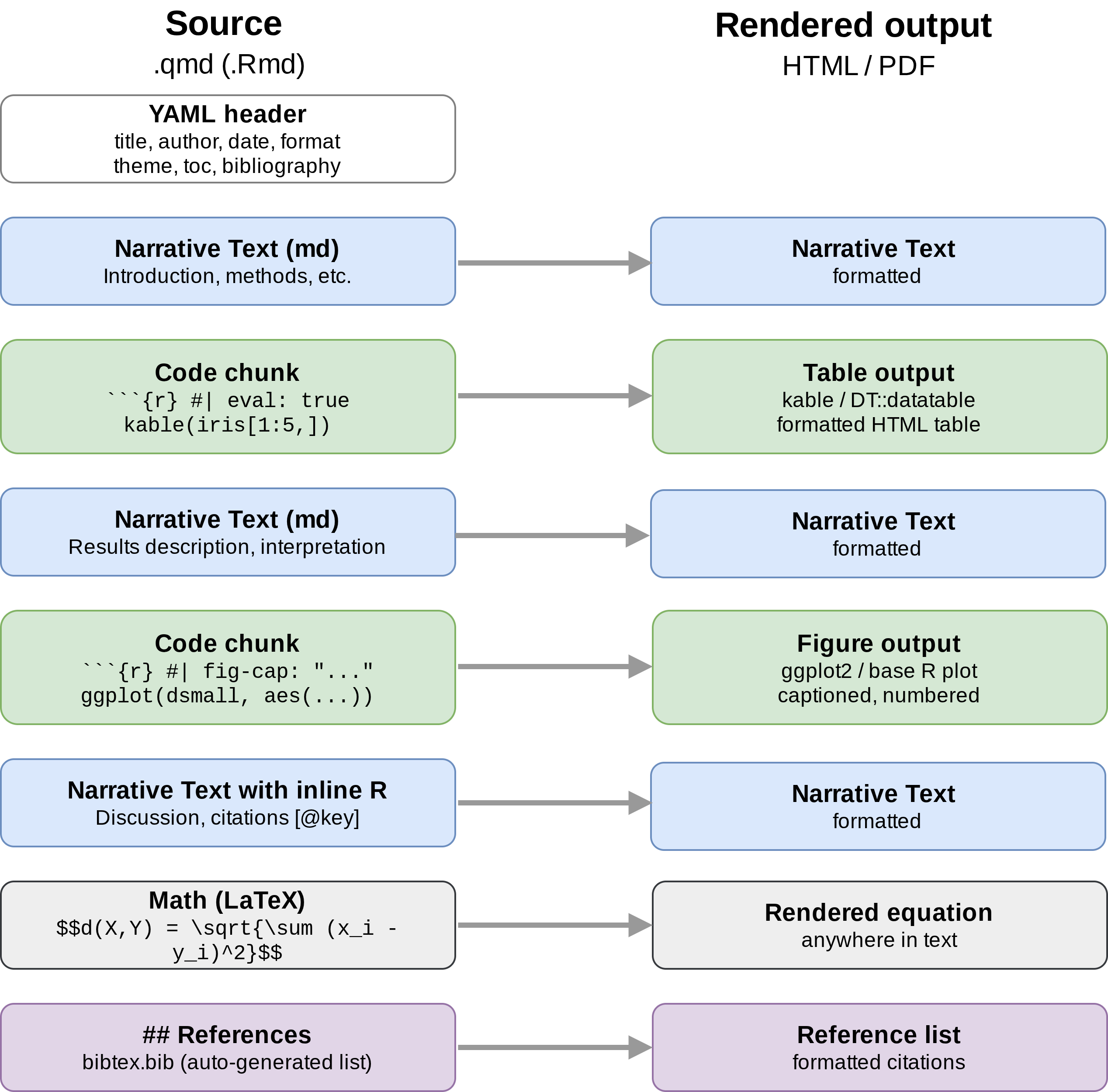
qmd/Rmd source files and the right panel the rendered output.Both systems share the same underlying toolchain: knitr executes the R code and pandoc converts the resulting Markdown to the final output format. This means that nearly everything learned for one system transfers directly to the other. Moreover, the syntax for both is very similar. Learning one in more details first makes it very easy to learn the other.
Quarto also supports Jupyter notebooks as an execution engine, making it suitable for Python and Julia workflows. .ipynb files can be rendered directly with quarto render notebook.ipynb, or a .qmd file can use the Jupyter engine by specifying jupyter: python3 in the YAML header. This makes Quarto a useful bridge for users working across R and Python environments. See the Quarto Python documentation for details.
Quarto
Install Quarto
Quarto is a standalone command-line tool that ships bundled with recent versions of RStudio (≥ 2022.07). For standalone installation or to update to the latest release, download the installer for your platform from https://quarto.org/docs/get-started/. The companion R package quarto provides convenience wrappers for rendering from within an R session.
To confirm that the Quarto CLI is available, run the following in a terminal.
Initialize a new .qmd script
Quarto source files use the .qmd extension. The simplest way to start is to copy an existing .qmd file (such as this tutorial) and adapt it. A minimal template and the shared Bibtex file are available here:
- Quarto sample script:
sample.qmd - Bibtex file for citations:
bibtex.bib
Metadata section
The YAML header of a .qmd file controls how the document is processed and rendered. It includes title, author, and date information as well as output format options. The following example produces a standalone HTML document with a floating table of contents and numbered sections, which is the recommended format for GEN242 course project reports.
---
title: "My First Quarto Document"
author: "Author: First Last"
date: last-modified
format:
  html:
    theme: default # try as alternatives: cosmo, flatly or lumen
    toc: true
    toc-depth: 3
    number-sections: true
    fig-cap-location: bottom
bibliography: bibtex.bib
---
Important settings in Quarto YAML header. For details see Options page here.
format:specifies the output format; the sub-key is the format name (e.g.html,pdf,docx)theme:specifes Quarto theme. Widely used arecosmo,flatlyandlumen. The Quarto HTML Themes page contains many additional examples.toc and toc-depth:Include table of contents and specify section levels (above #, ## and ###).- Option names use kebab-case (e.g.
toc-depth,number-sections) date: last-modifiedautomatically inserts the file modification date- To produce PDF output, replace
html:withpdf: - To generate multiple formats in one render pass, list them both under
format:
format:
  html:
    toc: true
  pdf:
    toc: true
Document-wide defaults for code chunk behaviour can be set under execute: in the YAML header, avoiding repetition across individual chunks:
---
execute:
  echo: true
  warning: false
  message: false
---
Render .qmd script
A Quarto document can be rendered from R, including nvim-R-Tmux, or from the command-line. In RStudio, the Render button triggers rendering.
From the command-line:
Markdown Formatting - Quick Reference
| Syntax | Result |
|---|---|
# Heading 1 / ## Heading 2 |
Section / subsection heading |
**bold** |
bold |
_italic_ |
italic |
- item |
Bullet list |
1. item |
Numbered list |
[@key] |
Citation |
[text](url) |
Hyperlink |
`code` |
Inline code |
$$...$$ |
Display math |
Full reference: https://quarto.org/docs/authoring/markdown-basics.html
Code chunks
Quarto code chunks are delimited by three backticks and a language identifier in curly braces. Chunk options are written as #| comment lines inside the chunk. This style works consistently across all execution engines (knitr and Jupyter) and is easier to read for long option lists. Note: Quarto will also render most code chunks correctly that are written in R Markdown (Rmd) style (see below).
The most important chunk options are:
eval: true/false— execute the chunkecho: true/false— show the source code in the outputwarning: false— suppress warningsmessage: false— suppress messagescache: true— cache results to speed up re-renderingfig-height: 4— figure height in inchesfig-width: 6— figure width in inchesfig-cap: "..."— figure captionlabel: fig-name— chunk label for cross-referencing (must start withfig-for figures)
For more details on chunk caching see the knitr cache documentation.
Learning Markdown
Quarto uses standard Markdown for prose. The syntax is minimal and easy to learn:
Tables
There are several ways to render tables. The knitr::kable function produces clean static tables, while the DT package produces fully interactive tables suitable for HTML output.
With knitr::kable
| Sepal.Length | Sepal.Width | Petal.Length | Petal.Width | Species |
|---|---|---|---|---|
| 5.1 | 3.5 | 1.4 | 0.2 | setosa |
| 4.9 | 3.0 | 1.4 | 0.2 | setosa |
| 4.7 | 3.2 | 1.3 | 0.2 | setosa |
| 4.6 | 3.1 | 1.5 | 0.2 | setosa |
| 5.0 | 3.6 | 1.4 | 0.2 | setosa |
| 5.4 | 3.9 | 1.7 | 0.4 | setosa |
| 4.6 | 3.4 | 1.4 | 0.3 | setosa |
| 5.0 | 3.4 | 1.5 | 0.2 | setosa |
| 4.4 | 2.9 | 1.4 | 0.2 | setosa |
| 4.9 | 3.1 | 1.5 | 0.1 | setosa |
| 5.4 | 3.7 | 1.5 | 0.2 | setosa |
| 4.8 | 3.4 | 1.6 | 0.2 | setosa |
With DT::datatable
A more powerful solution for HTML output is the DT package, which wraps the JavaScript DataTables library. The resulting tables can be sorted, filtered, and resized by the user.
JavaScript-dependent output such as DT::datatable can only be rendered to HTML, not PDF. This applies to both Quarto and R Markdown.
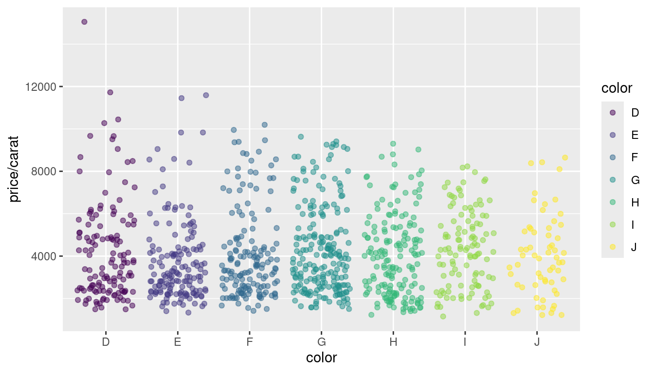
Figures
Plots generated by code chunks are automatically inserted in the output. Figure size is controlled with fig-height and fig-width chunk options.
library(ggplot2)
dsmall <- diamonds[sample(nrow(diamonds), 1000), ]
ggplot(dsmall, aes(color, price/carat)) + geom_jitter(alpha = I(1 / 2), aes(color=color))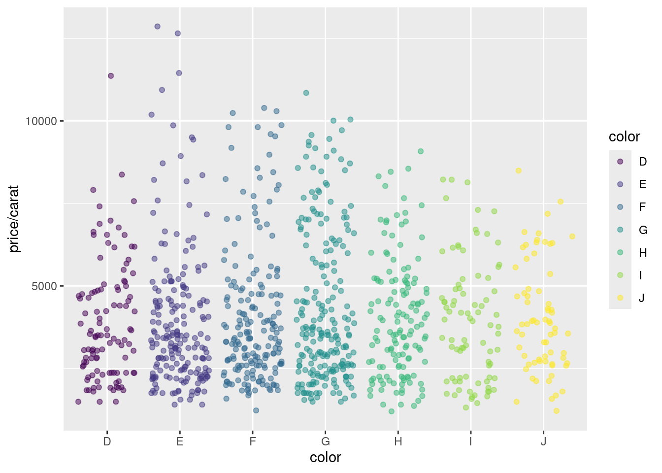
It is also possible to write a figure to a file explicitly and then insert it by referencing the file name with a markdown or html image link, such as . For additional details see the Quarto documentation here. This two-step approach is particularly useful in cases when figure generation is time-consuming, and thus real-time image generation during the rendering of Quarto or R Markdown documents becomes impractical.
Cross-referencing figures, tables and sections
Quarto has a native cross-referencing system. This works as follows: give a chunk a label starting with fig- and add a caption; then reference it anywhere in the document with @fig-label, which renders as a numbered hyperlink, here Figure 1. This name-based referencing scheme applies to tables (tbl- prefix) and sections (sec- prefix, requires number-sections: true). Before this extremely useful feature was only available in LaTeX (missing in R Markdown). Also note: for large documents, like PhD theses, where referencing of figures and tables across documents is important, this feature is best supported in Quarto Books. In this context it is also useful to know that Quarto documents can be converted to tex (LaTeX) files.
Custom functions
Custom functions can be kept in a separate R file and imported with source(). In the following example the file custom_Fct.R is sourced directly from GitHub.
Now the imported function (here myMAcomp) can be used.
myMA <- matrix(rnorm(100000), 10000, 10, dimnames=list(1:10000, paste("C", 1:10, sep="")))
resultDF <- myMAcomp(myMA=myMA, group=c(1,1,1,2,2,2,3,3,4,4), myfct=mean)
kable(resultDF[1:12,])| C1_C2_C3 | C4_C5_C6 | C7_C8 | C9_C10 |
|---|---|---|---|
| 1.0900599 | 0.0552483 | 0.2610207 | -0.1906031 |
| -0.7228645 | 0.4921195 | -0.9975280 | 0.2448808 |
| 0.1502273 | 0.3066726 | -1.7044671 | 0.6510076 |
| 0.0474822 | 0.1953876 | -0.3848315 | -0.3529045 |
| 0.2926998 | 0.9783578 | 0.5659983 | -2.0324317 |
| -0.2996951 | 0.5715911 | 0.0812536 | 0.6832752 |
| -0.2966968 | 0.2800871 | 0.6299184 | -1.6262742 |
| -0.0551971 | 0.0843747 | -0.3415473 | -0.2543040 |
| 0.3153155 | -0.5102449 | -0.4033627 | 0.9014025 |
| 0.0616046 | -0.0243732 | -0.4184517 | -0.4453049 |
| 0.8487860 | -0.5691444 | -0.0380007 | 1.2383162 |
| -0.8862990 | -0.3122685 | 0.8679277 | -0.0732828 |
Inline R code
To evaluate R code inline, enclose an R expression with a single backtick followed by r and then the expression. For instance, the back-ticked version of ‘r 1 + 1’ evaluates to 2 and ‘r pi’ evaluates to 3.1415927. Quarto also supports inline expressions for Python and Julia by replacing r with python or julia respectively, when those engines are active.
Mathematical equations
Standard LaTeX syntax is used for mathematical expressions. Single $ signs produce inline math, double $$ signs produce display math. For instance:
\[d(X,Y) = \sqrt[]{ \sum_{i=1}^{n}{(x_{i}-y_{i})^2} }\]
To learn LaTeX math syntax, consult the Wikibooks LaTeX tutorial or use an online equation editor such as this one.
Citations and bibliographies
Citations and bibliographies are handled via Bibtex. Reference collections are stored in a .bib file listed in the YAML header under bibliography:. To cite a publication, use the syntax [@key] where key is the identifier in the .bib file. For instance, [@Lawrence2013-kt] produces an inline citation (Lawrence et al. 2013) and adds the entry to the reference list at the end of the document. For general reference management and exporting references in Bibtex format, Paperpile is very helpful. For fine control over citation formatting, see the Quarto citations documentation.
Viewing a Quarto report on the HPCC cluster
Quarto HTML reports on UCR’s HPCC Cluster can be viewed in a local web browser by creating a symbolic link from the user’s .html directory. This way updates to the report appear immediately without copying the HTML file. For instance, if user ttest has rendered a report to ~/bigdata/today/quarto/sample.html, the link is created as follows:
The report is then accessible at https://cluster.hpcc.ucr.edu/~ttest/rmarkdown/sample.html. Access can be restricted with a password following the instructions here. To set up HTML viewing accounts, apply the configuration steps outlined on the HPCC website.
Viewing a Quarto report on GitHub
Quarto HTML files can be hosted and viewed on GitHub Pages. Follow the instructions here for the general workflow (public repos only). Quarto also has dedicated support via quarto publish gh-pages; see the Quarto publishing documentation for details.
Additional Quarto Features
The following Quarto features are mostly relevant for website design.
Callout blocks
Callout blocks highlight notes, warnings, tips, and important information in a visually distinct box. They are written with a fenced ::: div syntax.
::: {.callout-note}
This is a note. Use .callout-tip, .callout-warning, .callout-important,
or .callout-caution for other styles.
:::This is a note callout. Use .callout-tip, .callout-warning, .callout-important, or .callout-caution for other styles.
Callout blocks can also have titles: add ## My Title as the first line inside the block.
A title can be added by including a second-level heading as the first line inside the block:
Quarto projects and _quarto.yml
When a .qmd file is part of a larger website or book (such as the GEN242 course site), project-level settings are controlled by a _quarto.yml file in the root directory of the project. Individual .qmd files inherit these settings and only need to specify document-specific overrides in their own YAML headers. The GEN242 site _quarto.yml sets the sidebar, navigation, default theme, and bibliography, which is why the YAML headers of tutorial pages like this one are short.
Students writing course project reports as standalone files do not need a _quarto.yml and should include all required settings directly in the document YAML header.
A minimal _quarto.yml for a simple website looks like this:
project:
  type: website
  output-dir: docs

website:
  title: "My Site"
  navbar:
    left:
      - href: index.qmd
        text: Home

format:
  html:
    theme: cosmo
    toc: true
Additional Quarto resources
R Markdown
Simlarly as Quarto, R Markdown combines Markdown with embedded R code chunks. When compiled, the code is executed and its output is included in the final document alongside the prose. R Markdown documents (.Rmd files) can be rendered to HTML, PDF, Word, and other formats. The R code is processed by knitr and the resulting .md file is converted by pandoc to the final output. Historically, R Markdown is an extension of the older Sweave/LaTeX environment.
R Markdown remains widely used: most Bioconductor package vignettes are written in R Markdown, and a large fraction of published R analysis workflows use it. Students encountering Bioconductor documentation will therefore benefit from familiarity with R Markdown even though GEN242 course projects use Quarto.
Install R Markdown
Initialize a new .Rmd script
Template files for the following examples are available here:
- R Markdown sample script:
sample.Rmd - Bibtex file:
bibtex.bib
Download these files, open sample.Rmd in your preferred R IDE (e.g. RStudio, vim, or emacs), start an R session, and set the working directory to the folder containing both files.
Metadata section
The YAML header in an R Markdown script defines output format and rendering options. The BiocStyle:: prefix applies the formatting style of the BiocStyle package from Bioconductor.
---
title: "My First R Markdown Document"
author: "Author: First Last"
date: "Last update: 27 May, 2026"
output:
  BiocStyle::html_document:
    toc: true
    toc_depth: 3
    fig_caption: yes
fontsize: 14pt
bibliography: bibtex.bib
---
Render .Rmd script
An R Markdown script can be rendered with the render command or by pressing the Knit button in RStudio.
From the command-line:
A Makefile can also be used to render an .Rmd file. A sample Makefile is available here. Edit the MAIN variable (line 13) to the base name of the target .Rmd file, then run:
Code chunks
R code chunks are delimited by three backticks and {r}. Options are passed as comma-separated arguments on the opening line.
The most important chunk options are:
eval=TRUE/FALSE— execute the chunkecho=TRUE/FALSE— show the source codewarning=FALSE— suppress warningsmessage=FALSE— suppress messagescache=TRUE— cache resultsfig.height=4— figure height in inchesfig.width=6— figure width in inches
For more details see the R Markdown chunk options reference. Document-wide defaults can be set at the top of the script with:
Learning Markdown
Viewing an R Markdown report on the HPCC cluster
R Markdown reports on UCR’s HPCC Cluster can be viewed in a local web browser by creating a symbolic link from the user’s .html directory. For instance, if user ttest has rendered a report to ~/bigdata/today/rmarkdown/sample.html:
The report is then accessible at https://cluster.hpcc.ucr.edu/~ttest/rmarkdown/sample.html. See the HPCC website for instructions on setting up HTML viewing accounts.
Viewing an R Markdown report on GitHub
To host and view static HTML files on GitHub Pages, follow the instructions here. This works only with public GitHub repos.
Quarto vs R Markdown Comparison
Quarto and R Markdown share the same knitr/pandoc toolchain and identical support for Markdown prose, LaTeX math, Bibtex citations, knitr::kable, DT, and ggplot2. The table below summarises the key syntax differences for the features covered in this tutorial.
| Feature | Quarto (.qmd) |
R Markdown (.Rmd) |
|---|---|---|
| Output format key | format: html |
output: html_document |
| Option naming style | kebab-case: toc-depth |
underscore: toc_depth |
| Date | last-modified |
2026-05-27 19:40:55 as inline R |
| Chunk options | #\| eval: false inside chunk |
{r name, eval=FALSE} on opening line |
| Global chunk defaults | execute: block in YAML |
knitr::opts_chunk$set(...) in R chunk |
| Render from R | quarto::quarto_render("file.qmd") |
rmarkdown::render("file.Rmd") |
| Render from CLI | quarto render file.qmd |
Rscript -e "rmarkdown::render(...)" |
| Figure cross-refs | native via @fig-label |
requires bookdown output format |
| Callout blocks | ::: {.callout-note} |
not available |
| Multi-language chunks | R, Python, Julia, Observable natively | R only (Python via reticulate) |
| Project config | _quarto.yml |
_site.yml / _bookdown.yml |
| Inline R code | backtick + r + expr + backtick |
identical |
| Math, citations, Bibtex | [@key], $...$, $$...$$ |
identical |
Session Info
R version 4.5.1 (2025-06-13)
Platform: x86_64-pc-linux-gnu
Running under: Debian GNU/Linux 11 (bullseye)

Matrix products: default
BLAS:   /usr/lib/x86_64-linux-gnu/blas/libblas.so.3.9.0
LAPACK: /usr/lib/x86_64-linux-gnu/lapack/liblapack.so.3.9.0  LAPACK version 3.9.0

locale:
 [1] LC_CTYPE=en_US.UTF-8       LC_NUMERIC=C               LC_TIME=en_US.UTF-8        LC_COLLATE=en_US.UTF-8     LC_MONETARY=en_US.UTF-8    LC_MESSAGES=en_US.UTF-8    LC_PAPER=en_US.UTF-8       LC_NAME=C
 [9] LC_ADDRESS=C               LC_TELEPHONE=C             LC_MEASUREMENT=en_US.UTF-8 LC_IDENTIFICATION=C

time zone: America/Los_Angeles
tzcode source: system (glibc)

attached base packages:
[1] stats     graphics  grDevices utils     datasets  methods   base

other attached packages:
[1] ggplot2_4.0.2 knitr_1.51

loaded via a namespace (and not attached):
 [1] vctrs_0.7.3        cli_3.6.6          rlang_1.2.0        xfun_0.57          otel_0.2.0         generics_0.1.4     S7_0.2.1-1         jsonlite_2.0.0     glue_1.8.1         htmltools_0.5.9    scales_1.4.0
[12] rmarkdown_2.31     grid_4.5.1         tibble_3.3.1       evaluate_1.0.5     fastmap_1.2.0      yaml_2.3.12        lifecycle_1.0.5    compiler_4.5.1     dplyr_1.2.1        RColorBrewer_1.1-3 pkgconfig_2.0.3
[23] htmlwidgets_1.6.4  farver_2.1.2       digest_0.6.39      R6_2.6.1           tidyselect_1.2.1   dichromat_2.0-0.1  pillar_1.11.1      magrittr_2.0.5     withr_3.0.2        tools_4.5.1        gtable_0.3.6