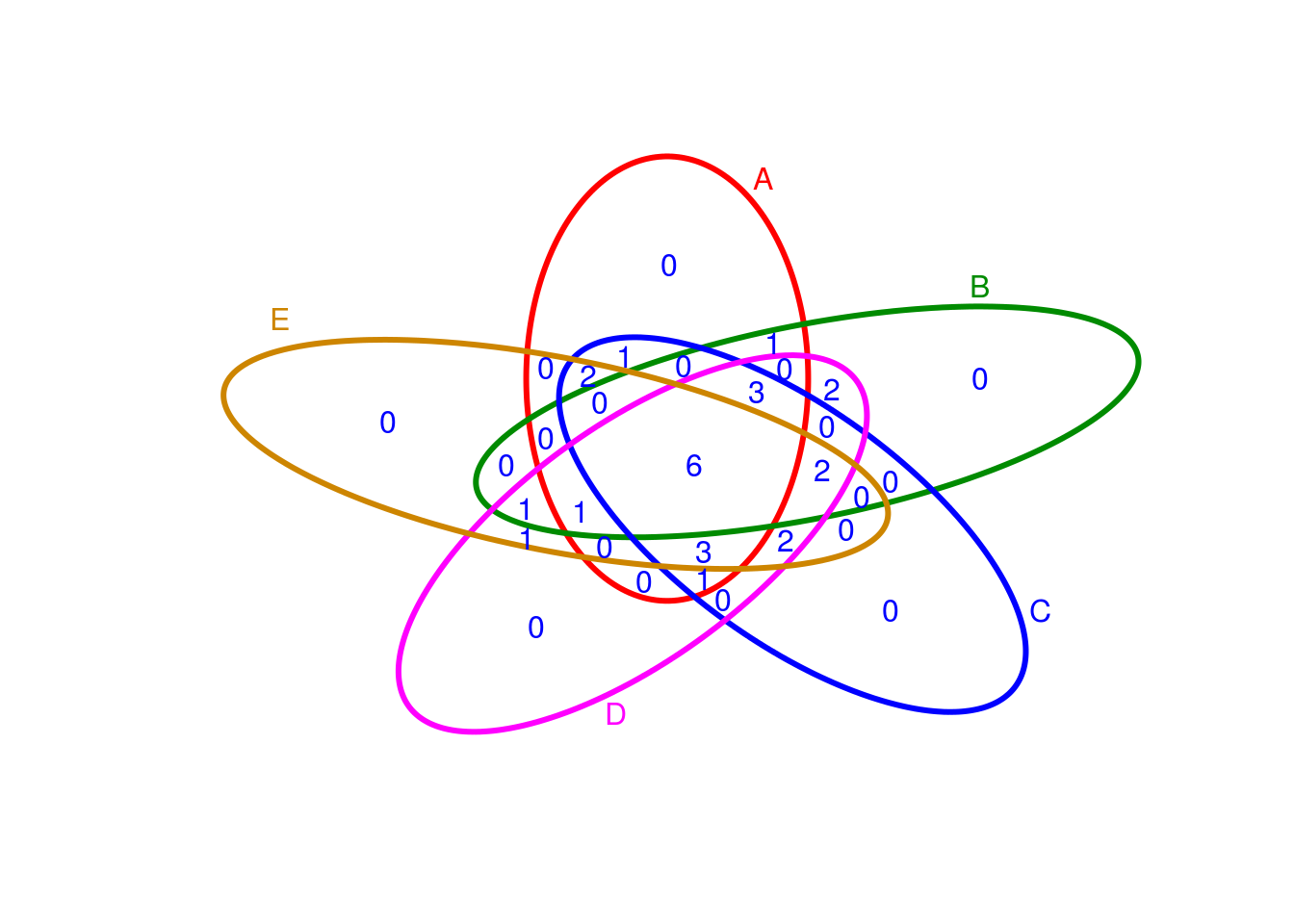
Venn Diagrams
library(systemPipeR)
setlist5 <- list(A=sample(letters, 18), B=sample(letters, 16), C=sample(letters, 20), D=sample(letters, 22), E=sample(letters, 18))
OLlist5 <- overLapper(setlist=setlist5, sep="_", type="vennsets")
vennPlot(OLlist5, mymain="", mysub="", colmode=2, ccol=c("blue", "red"))
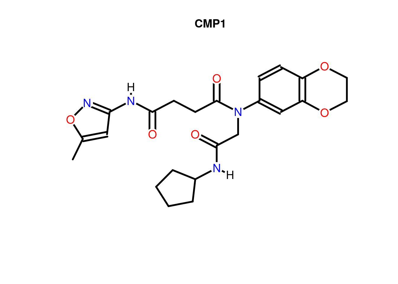
Compound Structures
Plots depictions of small molecules with ChemmineR package
library(ChemmineR)
data(sdfsample)
plot(sdfsample[1], print=FALSE)
ROC Plots
A variety of libraries are available for plotting receiver operating characteristic (ROC) curves in R:
Example
Most commonly, in an ROC we plot the true positive rate (y-axis) against the false positive rate (x-axis) at decreasing thresholds.
An illustrative example is provided in the ROCR package where one wants to inspect the content of the ROCR.simple object
defining the structure of the input data in two vectors.
# install.packages("ROCR") # Install if necessary on your laptop
library(ROCR)
data(ROCR.simple)
ROCR.simple
## $predictions
##   [1] 0.612547843 0.364270971 0.432136142 0.140291078 0.384895941 0.244415489 0.970641299
##   [8] 0.890172812 0.781781371 0.868751832 0.716680598 0.360168796 0.547983407 0.385240464
##  [15] 0.423739359 0.101699993 0.628095575 0.744769966 0.657732644 0.490119891 0.072369921
##  [22] 0.172741714 0.105722115 0.890078186 0.945548941 0.984667270 0.360180429 0.448687336
##  [29] 0.014823599 0.543533783 0.292368449 0.701561487 0.715459280 0.714985914 0.120604738
##  [36] 0.319672178 0.911723615 0.757325590 0.090988280 0.529402244 0.257402979 0.589909284
##  [43] 0.708412104 0.326672910 0.086546283 0.879459891 0.362693564 0.230157183 0.779771989
##  [50] 0.876086217 0.353281048 0.212014560 0.703293499 0.689075677 0.627012496 0.240911145
##  [57] 0.402801992 0.134794140 0.120473353 0.665444679 0.536339509 0.623494622 0.885179651
##  [64] 0.353777439 0.408939895 0.265686095 0.932159806 0.248500489 0.858876675 0.491735594
##  [71] 0.151350957 0.694457482 0.496513160 0.123504905 0.499788081 0.310718619 0.907651100
##  [78] 0.340078180 0.195097957 0.371936985 0.517308606 0.419560072 0.865639036 0.018527600
##  [85] 0.539086009 0.005422562 0.772728821 0.703885141 0.348213542 0.277656869 0.458674210
##  [92] 0.059045866 0.133257805 0.083685883 0.531958184 0.429650397 0.717845453 0.537091350
##  [99] 0.212404891 0.930846938 0.083048377 0.468610247 0.393378108 0.663367560 0.349540913
## [106] 0.194398425 0.844415442 0.959417835 0.211378771 0.943432189 0.598162949 0.834803976
## [113] 0.576836208 0.380396459 0.161874325 0.912325837 0.642933593 0.392173971 0.122284044
## [120] 0.586857799 0.180631658 0.085993218 0.700501359 0.060413627 0.531464015 0.084254795
## [127] 0.448484671 0.938583020 0.531006532 0.785213140 0.905121019 0.748438143 0.605235403
## [134] 0.842974300 0.835981859 0.364288579 0.492596896 0.488179708 0.259278968 0.991096434
## [141] 0.757364019 0.288258273 0.773336236 0.040906997 0.110241034 0.760726142 0.984599159
## [148] 0.253271061 0.697235328 0.620501132 0.814586047 0.300973098 0.378092079 0.016694412
## [155] 0.698826511 0.658692553 0.470206008 0.501489336 0.239143340 0.050999138 0.088450984
## [162] 0.107031842 0.746588080 0.480100183 0.336592126 0.579511087 0.118555284 0.233160827
## [169] 0.461150807 0.370549294 0.770178504 0.537336015 0.463227453 0.790240205 0.883431431
## [176] 0.745110673 0.007746305 0.012653524 0.868331219 0.439399995 0.540221346 0.567043171
## [183] 0.035815400 0.806543942 0.248707470 0.696702150 0.081439129 0.336315317 0.126480399
## [190] 0.636728451 0.030235062 0.268138293 0.983494405 0.728536415 0.739554341 0.522384507
## [197] 0.858970526 0.383807972 0.606960209 0.138387070
##
## $labels
##   [1] 1 1 0 0 0 1 1 1 1 0 1 0 1 0 0 0 1 1 1 0 0 0 0 1 0 1 0 0 1 1 0 1 1 1 0 0 1 1 0 1 0 1 0 1 0 1 0
##  [48] 1 0 1 1 0 1 0 1 0 0 0 0 1 1 1 1 0 0 0 1 0 1 0 0 1 0 0 0 0 0 0 0 0 1 0 1 0 0 1 1 0 0 1 0 0 1 0
##  [95] 1 0 1 1 0 1 0 0 0 1 0 0 1 0 0 1 1 1 0 0 0 1 1 0 0 1 0 0 1 0 1 0 0 1 1 1 1 1 0 1 1 0 0 0 0 1 1
## [142] 0 1 0 1 0 1 1 1 1 1 0 0 0 1 1 0 1 0 0 0 0 1 0 0 1 0 0 0 0 1 1 0 1 1 1 0 1 1 0 1 1 0 1 0 0 0 1
## [189] 0 0 0 1 0 1 1 0 1 0 1 0
pred <- prediction(ROCR.simple$predictions, ROCR.simple$labels)
perf <- performance( pred, "tpr", "fpr" )
plot(perf)
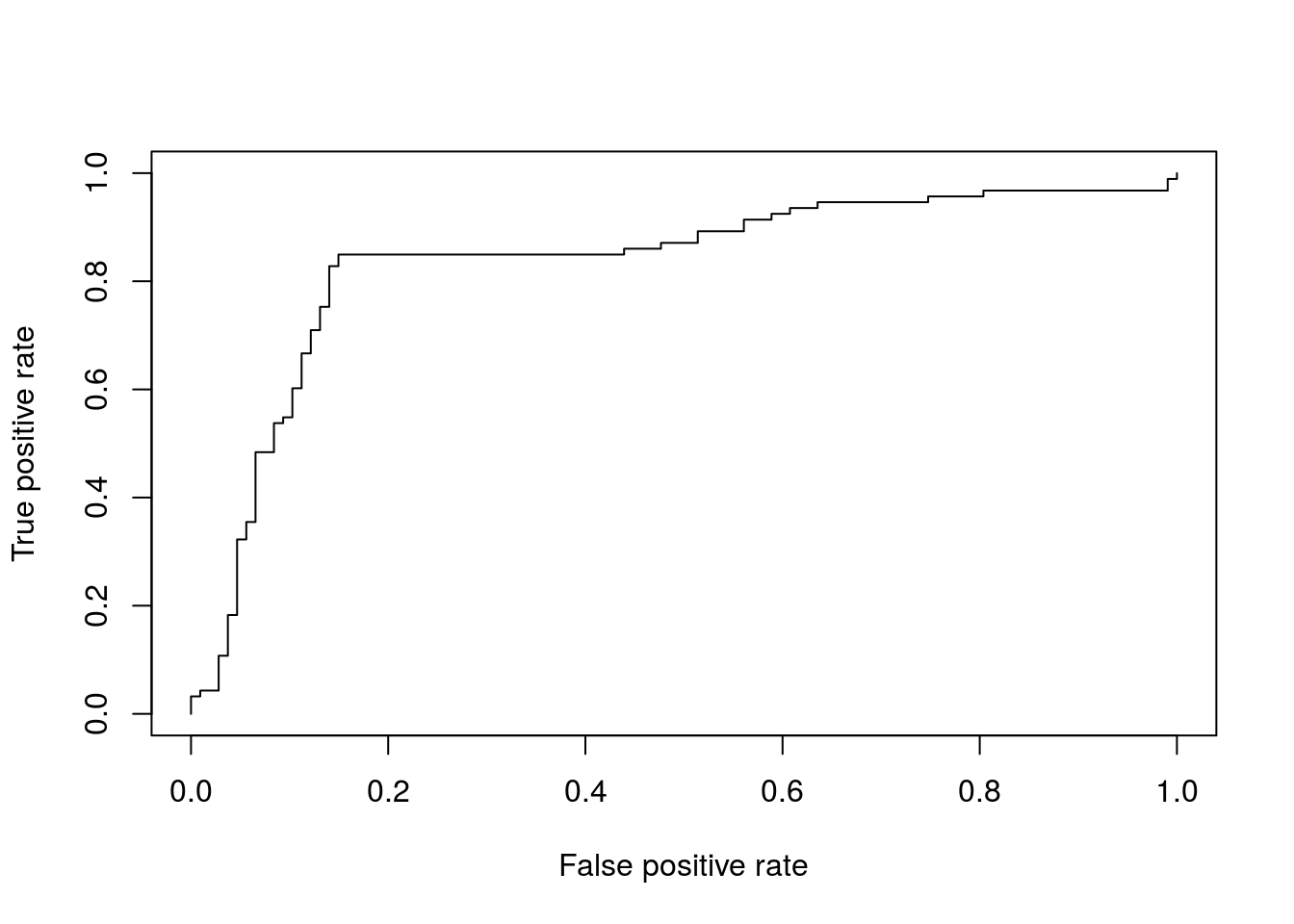
Obtain area under the curve (AUC)
auc <- performance( pred, "tpr", "fpr", measure = "auc")
auc@y.values[[1]]
## [1] 0.8341875
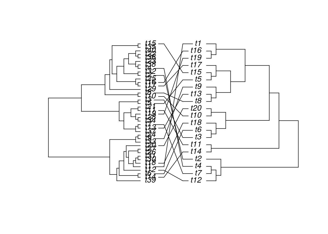
Trees
The ape package provides many useful utilities for phylogenetic analysis and tree plotting. Another useful package for
plotting trees is ggtree. The following example plots two trees face to face with links to identical
leaf labels.
library(ape)
tree1 <- rtree(40)
tree2 <- rtree(20)
association <- cbind(tree2$tip.label, tree2$tip.label)
cophyloplot(tree1, tree2, assoc = association,
            length.line = 4, space = 28, gap = 3)