Read counting with summarizeOverlaps in parallel mode using multiple cores
Reads overlapping with annotation ranges of interest are counted for
each sample using the summarizeOverlaps function (Lawrence et al., 2013). The read counting is
preformed for exonic gene regions in a non-strand-specific manner while
ignoring overlaps among different genes. Subsequently, the expression
count values are normalized by reads per kp per million mapped reads
(RPKM). The raw read count table (countDFeByg.xls) and the correspoding
RPKM table (rpkmDFeByg.xls) are written
to separate files in the directory of this project. Parallelization is
achieved with the BiocParallel package, here using 8 CPU cores.
library("GenomicFeatures"); library(BiocParallel)
txdb <- makeTxDbFromGFF(file="data/tair10.gff", format="gff", dataSource="TAIR", organism="Arabidopsis thaliana")
saveDb(txdb, file="./data/tair10.sqlite")
txdb <- loadDb("./data/tair10.sqlite")
(align <- readGAlignments(outpaths(args)[1])) # Demonstrates how to read bam file into R
eByg <- exonsBy(txdb, by=c("gene"))
bfl <- BamFileList(outpaths(args), yieldSize=50000, index=character())
multicoreParam <- MulticoreParam(workers=2); register(multicoreParam); registered()
counteByg <- bplapply(bfl, function(x) summarizeOverlaps(eByg, x, mode="Union",
                                               ignore.strand=TRUE,
                                               inter.feature=FALSE,
                                               singleEnd=TRUE))
countDFeByg <- sapply(seq(along=counteByg), function(x) assays(counteByg[[x]])$counts)
rownames(countDFeByg) <- names(rowRanges(counteByg[[1]])); colnames(countDFeByg) <- names(bfl)
rpkmDFeByg <- apply(countDFeByg, 2, function(x) returnRPKM(counts=x, ranges=eByg))
write.table(countDFeByg, "results/countDFeByg.xls", col.names=NA, quote=FALSE, sep="\t")
write.table(rpkmDFeByg, "results/rpkmDFeByg.xls", col.names=NA, quote=FALSE, sep="\t")
Sample of data slice of count table
read.delim("results/countDFeByg.xls", row.names=1, check.names=FALSE)[1:4,1:5]Sample of data slice of RPKM table
read.delim("results/rpkmDFeByg.xls", row.names=1, check.names=FALSE)[1:4,1:4]Note, for most statistical differential expression or abundance analysis
methods, such as edgeR or DESeq2, the raw count values should be used as input. The
usage of RPKM values should be restricted to specialty applications
required by some users, e.g. manually comparing the expression levels
among different genes or features.
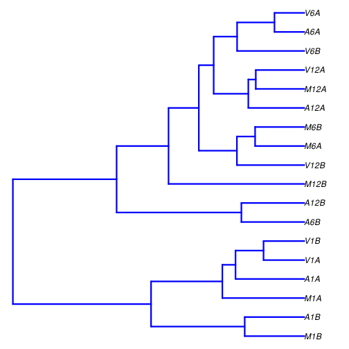
Sample-wise correlation analysis
The following computes the sample-wise Spearman correlation coefficients from
the rlog transformed expression values generated with the DESeq2 package. After
transformation to a distance matrix, hierarchical clustering is performed with
the hclust function and the result is plotted as a dendrogram
(also see file sample_tree.pdf).
library(DESeq2, quietly=TRUE); library(ape,  warn.conflicts=FALSE)
countDF <- as.matrix(read.table("./results/countDFeByg.xls"))
colData <- data.frame(row.names=targetsin(args)$SampleName, condition=targetsin(args)$Factor)
dds <- DESeqDataSetFromMatrix(countData = countDF, colData = colData, design = ~ condition)
d <- cor(assay(rlog(dds)), method="spearman")
hc <- hclust(dist(1-d))
png("results/sample_tree.pdf")
plot.phylo(as.phylo(hc), type="p", edge.col="blue", edge.width=2, show.node.label=TRUE, no.margin=TRUE)
dev.off()