Loading User Supplied PubChem BioAssay Data
This section demonstrates the process for creating a new bioactivity database from user supplied data. As an example, we will demonstrate the process of downloading an assay from the NCBI PubChem BioAssay bioactivity data repository, and loading this into a new database (Wang, et al., 2012).
First, get two files from PubChem BioAssay for the assay of interest: an XML file containing details on how the experiment was performed, and a CSV (comma separated value) file which contains the actual activity scores. For the purposes of this example, we will use the data from assay 1000, which is a confirmatory assay (titration assay) of 57 small molecules against a mevalonate kinase protein. More details on this assay were provided in the “Quick Tutorial,” where the same data is used. These files can be downloaded from PubChem BioAssay at http://pubchem.ncbi.nlm.nih.gov/ or loaded from the example data repository included in this package as follows:
library(bioassayR)
extdata_dir <- system.file("extdata", package="bioassayR")
assayDescriptionFile <- file.path(extdata_dir, "exampleAssay.xml")
activityScoresFile <- file.path(extdata_dir, "exampleScores.csv")
Next, create a new empty database for loading these data into. This example uses the R tempfile function to create the database in a random location. If you would like to keep your resulting database, replace myDatabaseFilename with your desired path and filename.
myDatabaseFilename <- tempfile()
mydb <- newBioassayDB(myDatabaseFilename, indexed=F)
We will also add a data source to this database, specifying that our data here mirrors an assay provided by PubChem BioAssay.
addDataSource(mydb, description="PubChem BioAssay", version="unknown")
The XML file provided by PubChem BioAssay contains extensive details on how the assay was performed, molecular targets, and results scoring methods. You can extract these using the parsePubChemBioassay function as follows.
The parsePubChemBioassay function also requires a .csv file which contains the activity scores for each assay, in the standard CSV format provided by PubChem BioAssay.
For data from sources other than PubChem BioAssay, you may need to write your own code to parse out the assay details- or type them in manually.
myAssay <- parsePubChemBioassay("1000", activityScoresFile, assayDescriptionFile)
myAssay
## class:		 bioassay
## aid:		 1000
## source_id:	 PubChem BioAssay
## assay_type:	 confirmatory
## organism:	 NA
## scoring:	 IC50
## targets:	 116516899
## target_types:	 protein
## total scores:	 57
Next, load the resulting data parsed from the XML and CSV files into the database. This creates records in the database for both the assay itself, and it’s molecular targets.
loadBioassay(mydb, myAssay)
To load additional assays, repeat the above steps. After all data is loaded, you can significantly improve subsequent query performance by adding an index to the database.
addBioassayIndex(mydb)
## Creating index: note this may take a long time for a large database
After indexing, perform a test query on your database to confirm that the data loaded correctly.
activeAgainst(mydb,"116516899")
##          fraction_active total_assays
## 16749973               1            1
## 16749974               1            1
## 16749975               1            1
## 16749976               1            1
## 16749977               1            1
## 16749978               1            1
## 16749979               1            1
## 16749980               1            1
## 16749981               1            1
## 16749982               1            1
## 16749983               1            1
## 16749984               1            1
## 16749985               1            1
## 16749986               1            1
## 16749987               1            1
## 16749988               1            1
## 16749989               1            1
## 16749990               1            1
## 16749991               1            1
## 16749992               1            1
## 16749993               1            1
## 16749994               1            1
## 16749995               1            1
## 16749996               1            1
## 16749997               1            1
## 16749998               1            1
## 16749999               1            1
## 16750000               1            1
## 16750001               1            1
## 16750002               1            1
## 16750003               1            1
## 16750004               1            1
## 16750005               1            1
## 16750006               1            1
## 16750007               1            1
## 16750016               1            1
Lastly, disconnect from the database to prevent data corruption.
disconnectBioassayDB(mydb)
Prebuilt Database Example: Investigate Activity of a Known Drug
A pre-built database containing large quantities of public domain bioactivity data sourced from the PubChem BioAssay database, can be downloaded from http://chemmine.ucr.edu/bioassayr.
While downloading the full database is recommended, it is possible to run this example using a small subset of the database, included within the bioassayR package for testing purposes.
This example demonstrates the utility of bioassayR for identifying the bioactivity patterns of a small drug-like molecule. In this example, we look at the binding activity patterns for the drug acetylsalicylic acid (aka Aspirin) and compare these binding data to annotated targets in the DrugBank drug database (Wishart, et al., 2008).
The DrugBank database is a valuable resource containing numerous data on drug activity in humans, including known molecular targets. In this exercise, first take a look at the
annotated molecular targets for acetylsalicylic acid by searching this name at http://drugbank.ca. This will provide a point of reference for comparing to the bioactivity
data we find in the prebuild PubChem BioAssay database. Note that DrugBank also contains the PubChem CID of this compound, which you can use to query the bioassayR PubChem BioAssay
database.
To get started first connect to the database. The variable sampleDatabasePath can be replaced with the filename of the full test database you downloaded, if you would like to use
that instead of the small example version included with this software package.
library(bioassayR)
extdata_dir <- system.file("extdata", package="bioassayR")
sampleDatabasePath <- file.path(extdata_dir, "sampleDatabase.sqlite")
pubChemDatabase <- connectBioassayDB(sampleDatabasePath)
Next, use the activeTargets function to find all protein targets which acetylsalicylic acid shows activity against in the loaded database.
These target IDs are NCBI Protein identifiers as provided by PubChem BioAssay (Tatusova, et al., 2014). In which cases do these results agree with or disagree
with the annotated targets from DrugBank?
drugTargets <- activeTargets(pubChemDatabase, "2244")
drugTargets
##           fraction_active total_screens
## 116241312            1.00             2
## 117144               1.00             1
## 166897622            1.00             1
## 317373262            1.00             1
## 3914304              1.00            14
## 3915797              0.75             8
## 548481               1.00            21
## 6686268              1.00             1
## 84028191             1.00             1
Now we would like to connect to the UniProt (Universal Protein Resource) database
to obtain annotation details on these targets
(Bateman, et al., 2015). The biomaRt Bioconductor package
is an excellent tool for this purpose, but works best with UniProt identifers,
instead of the NCBI Protein identifiers we currently have, so we must
translate the identifiers first (Durinck, et al., 2009; Durinck, et al., 2005).
We will use the translateTargetId function in bioassayR to obtain
a corresponding UniProt identifier for each NCBI Protein identifier (GI).
These identifier translations were obtained from UniProt and come pre-loaded
into the database. The translateTargetId takes only a single query and returns
one or more UniProt identifiers. Here we call it with sapply which automates
calling the function multiple times, one for each protein stored in drugTargets.
In many instances, a single query GI will translate into multiple UniProt
identifiers. In this case, we keep only the first one as the annotation
details we are looking for here will likely be the same for all of them.
# run translateTargetId on each target identifier
uniProtIds <- lapply(row.names(drugTargets), translateTargetId, database=pubChemDatabase, category="UniProt")

# if any targets had more than one UniProt ID, keep only the first one
uniProtIds <- sapply(uniProtIds, function(x) x[1])
Next, we connect to Ensembl via biomaRt to obtain a description for each
target that is a Homo sapiens gene. For more information,
consult the biomaRt documentation. After retrieving these data, we call the
match function to ensure they are in the same order as the query data.
library(biomaRt)
ensembl <- useEnsembl(biomart="ensembl",dataset="hsapiens_gene_ensembl")
proteinDetails <- getBM(attributes=c("description","uniprot_swissprot","external_gene_name"), filters=c("uniprot_swissprot"), mart=ensembl, values=uniProtIds)
proteinDetails <- proteinDetails[match(uniProtIds, proteinDetails$uniprot_swissprot),]
Now we can view this annotation data. NAs represent proteins not found
on the Homo sapiens Ensembl, which may be from other species.
proteinDetails
##                                                                                                                   description
## 2                                    cytochrome P450, family 3, subfamily A, polypeptide 4 [Source:HGNC Symbol;Acc:HGNC:2637]
## 1                                    cytochrome P450, family 1, subfamily A, polypeptide 2 [Source:HGNC Symbol;Acc:HGNC:2596]
## NA                                                                                                                       <NA>
## 5    prostaglandin-endoperoxide synthase 1 (prostaglandin G/H synthase and cyclooxygenase) [Source:HGNC Symbol;Acc:HGNC:9604]
## NA.1                                                                                                                     <NA>
## 6    prostaglandin-endoperoxide synthase 2 (prostaglandin G/H synthase and cyclooxygenase) [Source:HGNC Symbol;Acc:HGNC:9605]
## NA.2                                                                                                                     <NA>
## 4                                    cytochrome P450, family 2, subfamily C, polypeptide 9 [Source:HGNC Symbol;Acc:HGNC:2623]
## 3                                    cytochrome P450, family 2, subfamily D, polypeptide 6 [Source:HGNC Symbol;Acc:HGNC:2625]
##      uniprot_swissprot external_gene_name
## 2               P08684             CYP3A4
## 1               P05177             CYP1A2
## NA                <NA>               <NA>
## 5               P23219              PTGS1
## NA.1              <NA>               <NA>
## 6               P35354              PTGS2
## NA.2              <NA>               <NA>
## 4               P11712             CYP2C9
## 3               P10635             CYP2D6
Lastly, let’s again look at our active target list, with the annotation alongside.
Note, these only match up in length and order because in the above code
we removed all but one UniProt ID for each target protein, and then reordered
the biomaRt results with the match function to get them in the correct order.
drugTargets <- drugTargets[! is.na(proteinDetails[,1]),]
proteinDetails <- proteinDetails[!is.na(proteinDetails[,1]),]
cbind(proteinDetails, drugTargets)
##                                                                                                                description
## 2                                 cytochrome P450, family 3, subfamily A, polypeptide 4 [Source:HGNC Symbol;Acc:HGNC:2637]
## 1                                 cytochrome P450, family 1, subfamily A, polypeptide 2 [Source:HGNC Symbol;Acc:HGNC:2596]
## 5 prostaglandin-endoperoxide synthase 1 (prostaglandin G/H synthase and cyclooxygenase) [Source:HGNC Symbol;Acc:HGNC:9604]
## 6 prostaglandin-endoperoxide synthase 2 (prostaglandin G/H synthase and cyclooxygenase) [Source:HGNC Symbol;Acc:HGNC:9605]
## 4                                 cytochrome P450, family 2, subfamily C, polypeptide 9 [Source:HGNC Symbol;Acc:HGNC:2623]
## 3                                 cytochrome P450, family 2, subfamily D, polypeptide 6 [Source:HGNC Symbol;Acc:HGNC:2625]
##   uniprot_swissprot external_gene_name fraction_active total_screens
## 2            P08684             CYP3A4            1.00             2
## 1            P05177             CYP1A2            1.00             1
## 5            P23219              PTGS1            1.00             1
## 6            P35354              PTGS2            0.75             8
## 4            P11712             CYP2C9            1.00             1
## 3            P10635             CYP2D6            1.00             1
Identify Target Selective Compounds
In the previous example, acetylsalicylic acid was found to show binding activity against numerous proteins, including the COX-1 cyclooxygenase enzyme (NCBI Protein ID 166897622).
COX-1 activity is theorized to be the key mechanism in this molecules function as a nonsteroidal anti-inflammatory drug (NSAID).
In this example, we will look for other small molecules which selectively bind to COX-1, under the assumption that these may be worth further investigation as potential nonsteroidal anti-inflammatory drugs.
This example shows how bioassayR can be used
identify small molecules which selectively bind to a target of interest, and assist in the
discovery of small molecule drugs and molecular probes.
First, we will start by connecting to a database.
Once again, the variable sampleDatabasePath can be replaced with the filename of the full PubChem BioAssay database (downloadable from http://chemmine.ucr.edu/bioassayr), if you would like to use
that instead of the small example version included with this software package.
library(bioassayR)
extdata_dir <- system.file("extdata", package="bioassayR")
sampleDatabasePath <- file.path(extdata_dir, "sampleDatabase.sqlite")
pubChemDatabase <- connectBioassayDB(sampleDatabasePath)
The activeAgainst function can be used to show all small molecules in the database which demonstrate activity against COX-1 as follows.
Each row name represents a small molecule cid. The column labeled “total assays” shows the total number of times each small molecule has been screened against the target of interest. The column labeled “fraction active” shows the portion of these which were annotated as active as a number between 0 and 1.
This function allows users to consider different binding assays from distinct sources as replicates, to assist in distinguishing potentially spurious binding results from those with demonstrated reproducibility.
activeCompounds <- activeAgainst(pubChemDatabase, "166897622")
activeCompounds[1:10,] # look at the first 10 compounds
##        fraction_active total_assays
## 2244                 1            1
## 2662                 1            3
## 3033                 1            1
## 3194                 1            1
## 3672                 1            1
## 3715                 1            2
## 133021               1            2
## 247704               1            1
## 444899               1            1
## 445580               1            1
Looking only at compounds which show binding to the target of interest is not sufficient for identifying drug candidates, as a portion of these compounds may be target unselective compounds (TUCs) which bind
indiscriminately to a large number of distinct protein targets. The R function selectiveAgainst provides the user with a list of compounds that show activity against a target of interest (in at least one assay), while also showing limited activity against other targets.
The maxCompounds option limits the maximum number of results returned, and the minimumTargets
option limits returned compounds to those screened against a specified minimum of distinct targets. Results are formatted as a data.frame whereby each row name represents a distinct compound. The first column shows the number of distinct targets this compound shows activity against, and the second shows the total number of targets it was screened against.
selectiveCompounds <- selectiveAgainst(pubChemDatabase, "166897622",
    maxCompounds = 10, minimumTargets = 1)
selectiveCompounds
##          active_targets tested_targets
## 2662                  1              1
## 3033                  1              1
## 133021                1              1
## 11314954              1              1
## 13015959              1              1
## 44563999              1              1
## 44564000              1              1
## 44564001              1              1
## 44564002              1              1
## 44564003              1              1
In the example database these compounds are only showing one tested target because very few assays are loaded. Users are encouraged to try this example for themselves with the full PubChem BioAssay database downloadable from http://chemmine.ucr.edu/bioassayr for a more interesting and informative result.
Users can combine bioassayR with the ChemmineR library to obtain structural information on these target selective compounds, and then perform further analysis- such as structural clustering, visualization, and computing physicochemical properties.
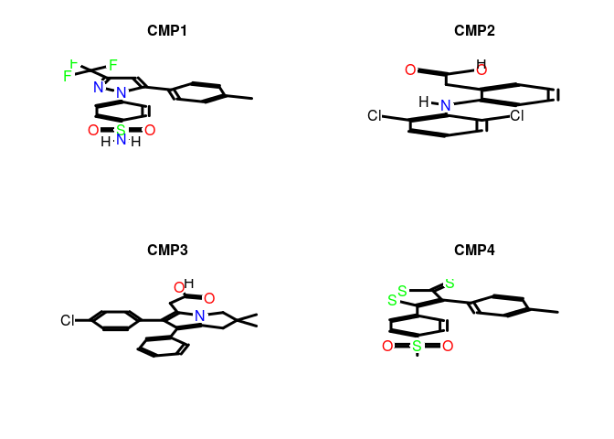
The ChemmineR software library can be used to download structural data for any of these compounds, and to visualize these structures as follows (Cao, et al., 2008).
This example requires an active internet connection, as the compound structures are obtained from a remote server.
library(ChemmineR)
structures <- getIds(as.numeric(row.names(selectiveCompounds)))
Here we visualize just the first four compounds found with selectiveAgainst. Consult the vignette supplied with ChemmineR for numerous examples of visualizing and analyzing these structures further.
plot(structures[1:4], print=FALSE) # Plots structures to R graphics device
Cluster Compounds by Activity Profile
This example demonstrates an example of clustering small molecules by similar bioactivity profiles across several distinct bioassay experiments.
In many cases it is too cpu and memory intensive to cluster all compounds in the database, so we first pull just a subset of these data from the database into an bioassaySet object, and then convert that into a compounds vs targets activity matrix for subsequent clustering according to similarities in activity profile.
The function getBioassaySetByCids extracts the activity data for a given list of compounds. Alternatively, the entire data for a given list of assay ids can be extracted with the function getAssays.
First, connect to the included sample database:
library(bioassayR)
extdata_dir <- system.file("extdata", package="bioassayR")
sampleDatabasePath <- file.path(extdata_dir, "sampleDatabase.sqlite")
sampleDB <- connectBioassayDB(sampleDatabasePath)
Next, select data from just 3 compounds to extract into a bioassaySet object for subsequent analysis.
compoundsOfInterest <- c("2244", "2662", "3715")
selectedAssayData <- getBioassaySetByCids(sampleDB, compoundsOfInterest)
selectedAssayData
## class:		 bioassaySet
## assays:		 1176
## compounds:	 3
## targets:	 453
## sources:	 bioassayR_testdata
The function perTargetMatrix converts the activity data extracted earlier into a matrix of targets (rows) vs compounds (columns). Data from multiple assays hitting the same target are summarized into a single value in the manner specified by the user. If you choose the summarizeReplicates option
activesFirst, any active scores take prescendence over inactives. If you choose the option mode the most abundant of either actives or inactives
is stored in the resulting matrix. You can also pass a custom function to decide how replicates are summarized.
In the resulting matrix a “2” represents an active compound vs target combination, a “1” represents an inactive combination, and a “0” represents
an untested or inconclusive combination. Inactive results can optionally be excluded from consideration
by passing the option inactives = FALSE. Here a sparse matrix (which omits actually storing 0 values) is used to save memory.
In a sparse matrix a period “.” entry is equal to a zero “0” entry, but is implied without
taking extra space in memory.
Here we create an activity matrix, choosing to include inactive values, and summarize replicates according to the statistical mode:
myActivityMatrix <- perTargetMatrix(selectedAssayData, inactives=TRUE, summarizeReplicates = "mode")
## Note: in this version active scores now use a 2 instead of a 1
myActivityMatrix[1:15,] # print the first 15 rows
## 15 x 3 sparse Matrix of class "dgCMatrix"
##           2244 2662 3715
## 548481       2    .    .
## 3914304      2    .    .
## 3915797      2    .    .
## 166897622    2    2    2
## 317373262    2    .    .
## 117144       2    .    .
## 6686268      2    .    .
## 84028191     2    .    .
## 116241312    2    .    .
## 73915100     1    .    .
## 160794       1    .    .
## 21464101     1    .    .
## 68565074     1    .    .
## 4325211      1    .    .
## 66528677     1    .    .
Next, we will re-create the activity matrix where protein targets
that are very similar at the sequence level (such as orthologues from different species)
are treated as replicates, and merged.
The function perTargetMatrix contains an option assayTargets
which let’s you specify the targets for each assay instead of taking them from the bioassaySet object.
The function assaySetTargets returns a vector of the targets for each assay
in a bioassaySet object, where the name of each element corresponds to it’s
assay identifier (aid). This is the format that must be passed to perTargetMatrix
to specify which assays are treated as replicates to be merged, so first we can
obtain these data, and then replace them with a custom merge criteria formatted
in the same manner.
myAssayTargets <- assaySetTargets(selectedAssayData)
myAssayTargets[1:5] # print the first 5 targets
##        410        411     624030        422        436
## "73915100"   "160794"   "160794" "21464101" "68565074"
The pre-built PubChem BioAssay database includes sequence level
protein target clustering results generated with the kClust tool
(options s=2.93, E-value < 1*10^-4, c=0.8) (Hauser, et al., 2013).
Each cluster has a unique number, and targets which cluster together are assigned
the same cluster number.
These clustering results are stored in the database as target
translations under category “kClust”. Now we will access these
traslations, and make a compound vs. target cluster matrix as follows.
# get kClust protein cluster number for a single target
translateTargetId(database = sampleDB, target = "166897622", category = "kClust")
## [1] NA
# get kClust protein cluster numbers for all targets in myAssayTargets
customMerge <- sapply(myAssayTargets, translateTargetId, database = sampleDB, category = "kClust")
customMerge[1:5]
##    410    411 624030    422    436
##     NA     NA     NA     NA     NA
mergedActivityMatrix <- perTargetMatrix(selectedAssayData, inactives=TRUE, assayTargets=customMerge)
## Note: in this version active scores now use a 2 instead of a 1
mergedActivityMatrix[1:15,] # print the first 15 rows
## 15 x 3 sparse Matrix of class "dgCMatrix"
##           2244 2662 3715
## 548481       2    .    .
## 3914304      2    .    .
## 3915797      2    .    .
## 166897622    2    2    2
## 317373262    2    .    .
## 117144       2    .    .
## 6686268      2    .    .
## 84028191     2    .    .
## 116241312    2    .    .
## 73915100     1    .    .
## 160794       1    .    .
## 21464101     1    .    .
## 68565074     1    .    .
## 4325211      1    .    .
## 66528677     1    .    .
Note that the merged matrix is smaller, because several similar protein targets
have been collapsed into single clusters.
# get number of rows and columns for unmerged matrix
dim(myActivityMatrix)
## [1] 298 3
# get number of rows and columns for merged matrix
dim(mergedActivityMatrix)
## [1] 298 3
Now, to make it possible to use binary clustering methods, we simplify the matrix
into a binary matrix where “1” represents active, and “0” represents either inactive
or untested combinations. We caution the user to carefully consider if this makes sense within the context of the specific experiments being analyzed.
binaryMatrix <- 1*(mergedActivityMatrix > 1)
binaryMatrix[1:15,] # print the first 15 rows
## 15 x 3 sparse Matrix of class "dgCMatrix"
##           2244 2662 3715
## 548481       1    .    .
## 3914304      1    .    .
## 3915797      1    .    .
## 166897622    1    1    1
## 317373262    1    .    .
## 117144       1    .    .
## 6686268      1    .    .
## 84028191     1    .    .
## 116241312    1    .    .
## 73915100     0    .    .
## 160794       0    .    .
## 21464101     0    .    .
## 68565074     0    .    .
## 4325211      0    .    .
## 66528677     0    .    .
As mentioned earlier, “0” and “.” entries in a sparse matrix are numerically equivalent.
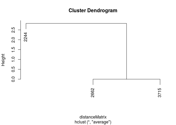
Cluster using the built in euclidean clustering functions within R to cluster.
This provides a dendrogram which indicates the similarity amongst compounds according to their activity profiles.
transposedMatrix <- t(binaryMatrix)
distanceMatrix <- dist(transposedMatrix)
clusterResults <- hclust(distanceMatrix, method="average")
plot(clusterResults)
A second way to compare activity profiles and cluster data is to pass
the activity matrix to the ChemmineR cheminformatics library as an FPset (binary fingerprint) object.
This represents the bioactivity data as a binary fingerprint (bioactivity fingerprint), which is a
binary string for each compound, where each bit represents activity (with a 1) or inactivity (with a 0) against
the full set of targets these compounds have shown activity against. This allows for pairwise comparison
of the bioactivity profile among compounds.
See the ChemmineR documentation at http://bioconductor.org/packages/ChemmineR/ for additional examples and details.
library(ChemmineR)
fpset <- bioactivityFingerprint(selectedAssayData)
## Note: in this version active scores now use a 2 instead of a 1
fpset
## An instance of a 453 bit "FPset" of type "bioactivity" with 3 molecules
Perform activity profile similarity searching with the FPset object, by comparing
the first compound to all compounds.
fpSim(fpset[1], fpset, method="Tanimoto")
## 2244 2662 3715
##  1.0  0.2  0.2
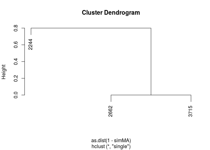
Compute an all-against-all bioactivity fingerprint similarity matrix for these compounds.
simMA <- sapply(cid(fpset), function(x) fpSim(fpset[x], fpset, sorted=FALSE, method="Tanimoto"))
simMA
##      2244 2662 3715
## 2244  1.0  0.2  0.2
## 2662  0.2  1.0  1.0
## 3715  0.2  1.0  1.0
Convert similarity matrix to a distance matrix and perform hierarcheal clustering.
clusterResults <- hclust(as.dist(1-simMA), method="single")
plot(clusterResults)
Finally, disconnect from the database.
disconnectBioassayDB(sampleDB)
Analyze and Load Raw Screening Data
This example demonstrates the basics of analyzing and loading data
from a high throughput screening experiment with scores for 21,888
distinct compounds.
This example is based on the cellHTS2 library
(Boutros, et al., 2006). Example data
is used which is included with cellHTS2. This is actually data from
screening dsRNA against live cells, however we will treat it as small molecule
binding data against a protein target as the data format is the same.
First read in the screening data provided with cellHTS2.
library(cellHTS2)
library(bioassayR)

dataPath <- system.file("KcViab", package="cellHTS2")
x <- readPlateList("Platelist.txt",
                   name="KcViab",
                   path=dataPath)

x <- configure(x,
               descripFile="Description.txt",
               confFile="Plateconf.txt",
               logFile="Screenlog.txt",
               path=dataPath)

xn <- normalizePlates(x,
                      scale="multiplicative",
                      log=FALSE,
                      method="median",
                      varianceAdjust="none")
Next, score and summarize the replicates.
xsc <- scoreReplicates(xn, sign="-", method="zscore")
xsc <- summarizeReplicates(xsc, summary="mean")
Parse the annotation data.
xsc <- annotate(xsc, geneIDFile="GeneIDs_Dm_HFA_1.1.txt", path=dataPath)
Apply a sigmoidal transformation to generate binary calls.
y <- scores2calls(xsc, z0=1.5, lambda=2)
binaryCalls <- round(Data(y))
Convert the binary calls into an activity table that bioassayR can parse.
scoreDataFrame <- cbind(geneAnno(y), binaryCalls)
rawScores <- as.vector(Data(xsc))
rawScores <- rawScores[wellAnno(y) == "sample"]
scoreDataFrame <- scoreDataFrame[wellAnno(y) == "sample",]
activityTable <- cbind(cid=scoreDataFrame[,1],
     activity=scoreDataFrame[,2], score=rawScores)
activityTable <- as.data.frame(activityTable)
activityTable[1:10,]
##        cid activity              score
## 1  CG11371        1     2.147814893189
## 2  CG31671        1   4.00105151825918
## 3  CG11376        0  0.955550327380792
## 4  CG11723        0  0.768879954745058
## 5  CG12178        0   1.12105534792054
## 6   CG7261        0 -0.126481089856157
## 7   CG2674        0  0.706942495432899
## 8   CG7263        0  0.920455054477106
## 9   CG4822        0  0.251440513724104
## 10  CG4265        0  0.414137389305878
Create a new (temporary in this case) bioassayR database to load these data into.
myDatabaseFilename <- tempfile()
mydb <- newBioassayDB(myDatabaseFilename, indexed=F)
addDataSource(mydb, description="other", version="unknown")
Create an assay object for the new assay.
myAssay <- new("bioassay",aid="1", source_id="other",
     assay_type="confirmatory", organism="unknown", scoring="activity rank",
     targets="2224444", target_types="protein", scores=activityTable)
Load this assay object into the bioassayR database.
loadBioassay(mydb, myAssay)
mydb
## class:		 BioassayDB
## assays:		 1
## sources:	 other
## writeable:	yes
Now that these data are loaded, you can use them to perform any of the other analysis examples in this document.
Lastly, for the purposes of this example, disconnect from the example database.
disconnectBioassayDB(mydb)
Custom SQL Queries
While many pre-built queries are provided (see other examples and man pages)
advanced users can also build their own SQL queries.
As bioassayR uses a SQLite database, you can consult http://www.sqlite.org for specifics on building SQL queries.
We also reccomend the book “Using SQLite” (Kreibich, 2010).
To get started first connect to a database. If you downloaded the full PubChem BioAssay
database from the authors website, the variable sampleDatabasePath can be replaced with the filename of the database you downloaded, if you would like to use
that instead of the small example version included with this software package.
library(bioassayR)
extdata_dir <- system.file("extdata", package="bioassayR")
sampleDatabasePath <- file.path(extdata_dir, "sampleDatabase.sqlite")
pubChemDatabase <- connectBioassayDB(sampleDatabasePath)
First you will want to see the structure
of the database as follows:
queryBioassayDB(pubChemDatabase, "SELECT * FROM sqlite_master WHERE type='table'")
##    type               name           tbl_name rootpage
## 1 table           activity           activity        2
## 2 table             assays             assays        3
## 3 table            domains            domains        4
## 4 table            sources            sources        5
## 5 table            targets            targets        6
## 6 table targetTranslations targetTranslations       99
##                                                                                                  sql
## 1     CREATE TABLE activity (aid INTEGER, cid INTEGER, sid INTEGER, activity INTEGER, score INTEGER)
## 2 CREATE TABLE assays (source_id INTEGER, aid INTEGER, assay_type TEXT, organism TEXT, scoring TEXT)
## 3                                                CREATE TABLE domains (domain TEXT, ta rget INTEGER)
## 4           CREATE TABLE sources (source_id INTEGER PRIMARY KEY ASC, description TEXT, version TEXT)
## 5                                  CREATE TABLE targets (aid INTEGER, target TEXT, target_type TEXT)
## 6                      CREATE TABLE targetTranslations (target TEXT, category TEXT, identifier TEXT)
For example, you can find the first 10 assays a given compound has participated in as follows:
queryBioassayDB(pubChemDatabase, "SELECT DISTINCT(aid) FROM activity WHERE cid = '2244' LIMIT 10")
##    aid
## 1    1
## 2  103
## 3  105
## 4  107
## 5  109
## 6  113
## 7  115
## 8  119
## 9  121
## 10 123
This example prints the activity scores from a specified assay:
queryBioassayDB(pubChemDatabase, "SELECT * FROM activity WHERE aid = '393818'")
##      aid      cid       sid activity score
## 1 393818     3672 103174500        1    NA
## 2 393818     2662 103181002        1    NA
## 3 393818 25258347 103594370       NA    NA
## 4 393818 25258348 103594371        1    NA
## 5 393818 25258349 103594372        1    NA
## 6 393818 25258350 103594373        1    NA
A NATURAL JOIN automatically merges tables which share common rows, making
it easier to parse data spread across many tables. Here we merge the activity
table (raw scores), with the assay table (assay annotation details) and the
protein targets table:
queryBioassayDB(pubChemDatabase, "SELECT * FROM activity NATURAL JOIN assays NATURAL JOIN targets WHERE cid = '2244' LIMIT 10")
##    aid  cid      sid activity score source_id   assay_type organism
## 1  410 2244 11110749        0     0         1 confirmatory     <NA>
## 2  411 2244 11110749        0     0         1 confirmatory     <NA>
## 3  422 2244 17404602        0    -6         1    screening     <NA>
## 4  436 2244 17404602        0     5         1    screening     <NA>
## 5  445 2244 11110749        0     0         1 confirmatory     <NA>
## 6  445 2244 11110749        0     0         1 confirmatory     <NA>
## 7  445 2244 11110749        0     0         1 confirmatory     <NA>
## 8  445 2244 11110749        0     0         1 confirmatory     <NA>
## 9  445 2244 11110749        0     0         1 confirmatory     <NA>
## 10 445 2244 11110749        0     0         1 confirmatory     <NA>
##    scoring   target target_type
## 1     <NA> 73915100     protein
## 2  Potency   160794     protein
## 3     <NA> 21464101     protein
## 4     <NA> 68565074     protein
## 5     <NA> 10092619     protein
## 6     <NA> 10092619     protein
## 7     <NA> 10092619     protein
## 8     <NA> 10092619     protein
## 9     <NA> 10092619     protein
## 10    <NA> 10092619     protein
Lastly, disconnecting from the database after analysis reduces the chances of data corruption. If you are using a pre-built database in read only mode (as demonstrated in the Prebuilt Database Example section) you can optionally skip this step, as only writable databases are prone to corruption from failure to disconnect.
disconnectBioassayDB(pubChemDatabase)