systemPipeR: Workflow design and reporting generation environment
24 minute read
Introduction
systemPipeR
is provides flexible utilities for building and running automated end-to-end
analysis workflows for a wide range of research applications, including
next-generation sequencing (NGS) experiments, such as RNA-Seq, ChIP-Seq,
VAR-Seq and Ribo-Seq (H Backman and Girke 2016). Important features include a uniform
workflow interface across different data analysis applications, automated
report generation, and support for running both R and command-line software,
such as NGS aligners or peak/variant callers, on local computers or compute
clusters (Figure 1). The latter supports interactive job submissions and batch
submissions to queuing systems of clusters. For instance, systemPipeR can
be used with any command-line aligners such as BWA (Heng Li 2013; H. Li and Durbin 2009),
HISAT2 (Kim, Langmead, and Salzberg 2015), TopHat2 (Kim et al. 2013) and Bowtie2
(Langmead and Salzberg 2012), as well as the R-based NGS aligners
Rsubread
(Liao, Smyth, and Shi 2013) and gsnap (gmapR)
(Wu and Nacu 2010). Efficient handling of complex sample sets (e.g. FASTQ/BAM
files) and experimental designs are facilitated by a well-defined sample
annotation infrastructure which improves reproducibility and user-friendliness
of many typical analysis workflows in the NGS area (Lawrence et al. 2013).
The main motivation and advantages of using systemPipeR for complex data analysis tasks are:
- Facilitates the design of complex data analysis workflows
- Consistent workflow interface for different large-scale data types
- Makes NGS analysis with Bioconductor utilities more accessible to new users
- Simplifies usage of command-line software from within R
- Reduces the complexity of using compute clusters for R and command-line software
- Accelerates runtime of workflows via parallelization on computer systems with multiple CPU cores and/or multiple compute nodes
- Improves reproducibility by automating analyses and generation of analysis reports
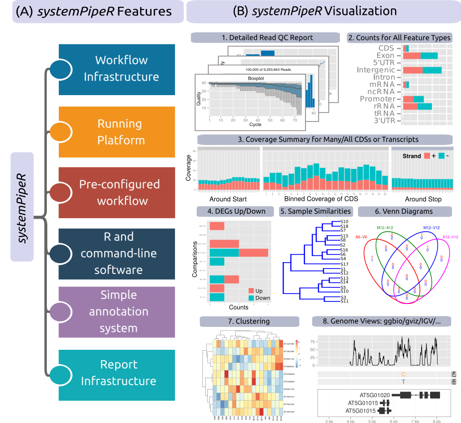
Figure 1: Relevant features in systemPipeR.
Workflow design concepts are illustrated under (A & B). Examples of
systemPipeR’s visualization functionalities are given under (C).
A central concept for designing workflows within the systemPipeR
environment is the use of workflow management containers. They support
the widely used community standard Common Workflow Language
(CWL) for describing analysis workflows in a generic and reproducible manner, introducing
SYSargs2 workflow control class (see Figure 2). Using this community
standard in systemPipeR has many advantages. For instance, the integration
of CWL allows running systemPipeR workflows from a single specification
instance either entirely from within R, from various command-line wrappers
(e.g., cwl-runner) or from other languages (, e.g., Bash or Python).
systemPipeR includes support for both command-line and R/Bioconductor
software as well as resources for containerization, parallel evaluations on
computer clusters along with the automated generation of interactive analysis
reports.
An important feature of systemPipeR's CWL interface is that it provides two
options to run command-line tools and workflows based on CWL. First, one can
run CWL in its native way via an R-based wrapper utility for cwl-runner or
cwl-tools (CWL-based approach). Second, one can run workflows using CWL’s
command-line and workflow instructions from within R (R-based approach). In the
latter case the same CWL workflow definition files (e.g. *.cwl and *.yml)
are used but rendered and executed entirely with R functions defined by
systemPipeR, and thus use CWL mainly as a command-line and workflow
definition format rather than execution software to run workflows. In this regard
systemPipeR also provides several convenience functions that are useful for
designing and debugging workflows, such as a command-line rendering function to
retrieve the exact command-line strings for each data set and processing step
prior to running a command-line.
This overview introduces the design of a new CWL S4 class in systemPipeR,
as well as the custom command-line interface, combined with the overview of all
the common analysis steps of NGS experiments.
Workflow design structure using SYSargs2
The flexibility of systemPipeR's workflow control class scales to any
number of analysis steps necessary in a workflow. This can include
variable combinations of steps requiring command-line or R-based software executions.
The connectivity among all workflow steps is achieved by the SYSargs2 workflow
control class (see Figure 3). This S4 class is a list-like container where
each instance stores all the input/output paths and parameter components
required for a particular data analysis step. SYSargs2 instances are
generated by two constructor functions, loadWorkflow and renderWF, using as
data input so called targets or yaml files as well as two cwl parameter files (for
details see below). When running preconfigured workflows, the only input the
user needs to provide is the initial targets file containing the paths to the
input files (e.g. FASTQ) along with unique sample labels. Subsequent targets
instances are created automatically. The parameters required for running
command-line software is provided by the parameter (.cwl) files described
below.
To support one or many workflow steps in a single container the SYSargsList class
capturing all information required to run, control and monitor complex workflows from
start to finish.
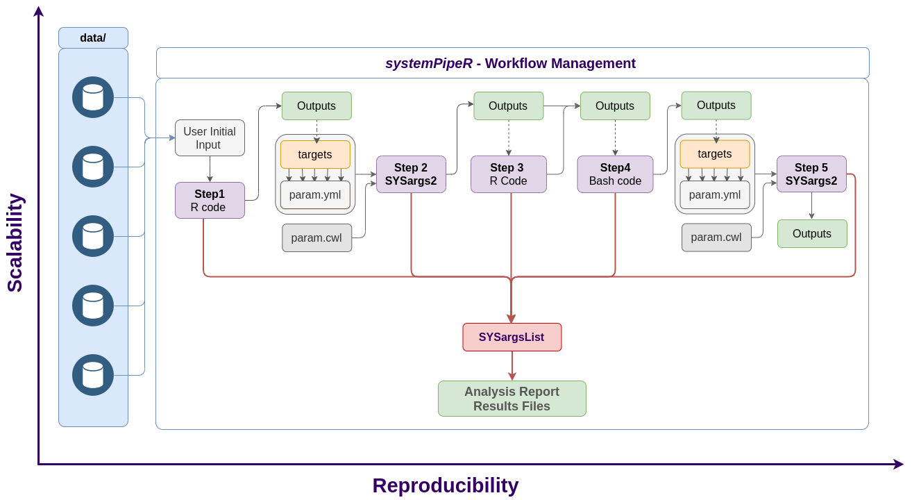
Figure 2: Workflow steps with input/output file operations are controlled by
SYSargs2 objects. Each SYSargs2 instance is constructed from one targets
and two param files. The only input provided by the user is the initial targets
file. Subsequent targets instances are created automatically, from the previous
output files. Any number of predefined or custom workflow steps are supported. One
or many SYSargs2 objects are organized in an SYSargsList container.
Workflow Management with SYSargsList
In systemPipeR allows to create (multi-step analyses) and run workflows directly from R or the command-line using local systems, HPC cluster or cloud platforms.
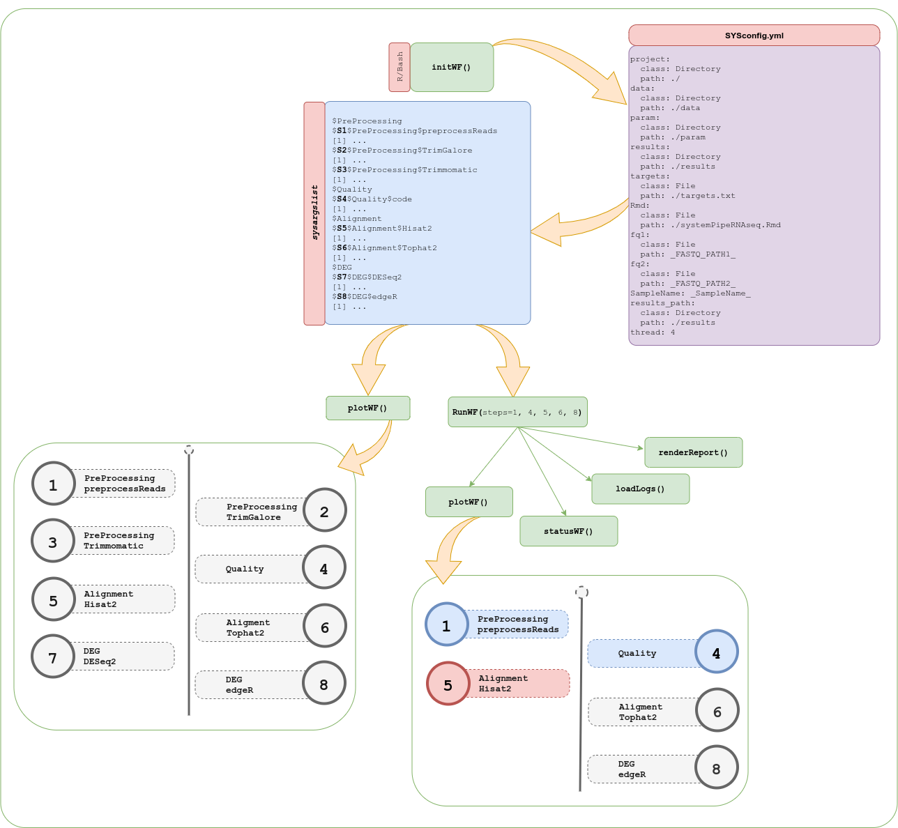
Figure 3: Workflow Management using SYSargsList.
Getting Started
Installation
The R software for running
systemPipeR
can be downloaded from CRAN. The
systemPipeR environment can be installed from the R console using the
BiocManager::install
command. The associated data package
systemPipeRdata
can be installed the same way. The latter is a helper package for generating
systemPipeR workflow environments with a single command containing all
parameter files and sample data required to quickly test and run workflows.
if (!requireNamespace("BiocManager", quietly = TRUE)) install.packages("BiocManager")
BiocManager::install("systemPipeR")
BiocManager::install("systemPipeRdata")
Please note that if you desire to use a third-party command line tool, the particular tool and dependencies need to be installed and executable. See details.
Loading package and documentation
library("systemPipeR")  # Loads the package
library(help = "systemPipeR")  # Lists package info
vignette("systemPipeR")  # Opens vignette
Load sample data and workflow templates
The mini sample FASTQ files used by this overview vignette as well as the
associated workflow reporting vignettes can be loaded via the
systemPipeRdata package as shown below. The chosen data set
SRP010938 obtains 18
paired-end (PE) read sets from Arabidposis thaliana (Howard et al. 2013). To
minimize processing time during testing, each FASTQ file has been subsetted to
90,000-100,000 randomly sampled PE reads that map to the first 100,000
nucleotides of each chromosome of the A. thalina genome. The corresponding
reference genome sequence (FASTA) and its GFF annotation files (provided in the
same download) have been truncated accordingly. This way the entire test sample
data set requires less than 200MB disk storage space. A PE read set has been
chosen for this test data set for flexibility, because it can be used for
testing both types of analysis routines requiring either SE (single-end) reads
or PE reads.
The following generates a fully populated systemPipeR workflow environment
(here for RNA-Seq) in the current working directory of an R session. At this time
the package includes workflow templates for RNA-Seq, ChIP-Seq, VAR-Seq, and Ribo-Seq.
Templates for additional NGS applications will be provided in the future.
Directory structure
The working environment of the sample data loaded in the previous step contains the following pre-configured directory structure (Figure 4). Directory names are indicated in green. Users can change this structure as needed, but need to adjust the code in their workflows accordingly.
- workflow/ (e.g. rnaseq/)
- This is the root directory of the R session running the workflow.
- Run script ( *.Rmd) and sample annotation (targets.txt) files are located here.
- Note, this directory can have any name (e.g. rnaseq, varseq). Changing its name does not require any modifications in the run script(s).
- Important subdirectories:
- param/
- Stores non-CWL parameter files such as: *.param, *.tmpl and *.run.sh. These files are only required for backwards compatibility to run old workflows using the previous custom command-line interface.
- param/cwl/: This subdirectory stores all the CWL parameter files. To organize workflows, each can have its own subdirectory, where all
CWL paramandinput.ymlfiles need to be in the same subdirectory.
- data/
- FASTQ files
- FASTA file of reference (e.g. reference genome)
- Annotation files
- etc.
- results/
- Analysis results are usually written to this directory, including: alignment, variant and peak files (BAM, VCF, BED); tabular result files; and image/plot files
- Note, the user has the option to organize results files for a given sample and analysis step in a separate subdirectory.
- param/
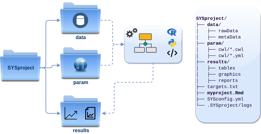
Figure 5: systemPipeR’s preconfigured directory structure.
The following parameter files are included in each workflow template:
targets.txt: initial one provided by user; downstreamtargets_*.txtfiles are generated automatically*.param/cwl: defines parameter for input/output file operations, e.g.:hisat2-se/hisat2-mapping-se.cwlhisat2-se/hisat2-mapping-se.yml
*_run.sh: optional bash scripts- Configuration files for computer cluster environments (skip on single machines):
.batchtools.conf.R: defines the type of scheduler forbatchtoolspointing to template file of cluster, and located in user’s home directory*.tmpl: specifies parameters of scheduler used by a system, e.g. Torque, SGE, Slurm, etc.
Structure of targets file
The targets file defines all input files (e.g. FASTQ, BAM, BCF) and
sample comparisons of an analysis workflow. The following shows the format of a
sample targets file included in the package. It also can be viewed and
downloaded from systemPipeR’s GitHub repository
here.
In a target file with a single type of input files, here FASTQ files of
single-end (SE) reads, the first three columns are mandatory including their
column names, while it is four mandatory columns for FASTQ files of PE reads.
All subsequent columns are optional and any number of additional columns can be
added as needed. The columns in targets files are expected to be tab separated (TSV format).
The SampleName column contains usually short labels for
referencing samples (here FASTQ files) accross many workflow steps (e.g.
plots and column titles). Importantly, the labels used in the SampleName
column need to be unique, while technical or biological replicates are
indicated by duplicated values under the Factor column. For readability
and transparency, it is useful to use here a short, consistent and informative
syntax for naming samples and replicates. To avoid problems with other
packages or external software, it is recommended to use the basic naming rules
for R objects and their components as outlined here.
This is important since the values used under the SampleName and Factor
columns are intended to be used as labels for naming columns or plotting features
in downstream analysis steps.
Users should note here, the usage of targets files is optional when using systemPipeR’s new CWL interface. They can be replaced by a standard YAML input file used by CWL. Since for organizing experimental variables targets files are extremely useful and user-friendly. Thus, we encourage users to keep using them.
Structure of targets file for single-end (SE) samples
library(systemPipeR)
targetspath <- system.file("extdata", "targets.txt", package = "systemPipeR")
read.delim(targetspath, comment.char = "#")[1:4, ]
##                      FileName SampleName Factor SampleLong Experiment
## 1 ./data/SRR446027_1.fastq.gz        M1A     M1  Mock.1h.A          1
## 2 ./data/SRR446028_1.fastq.gz        M1B     M1  Mock.1h.B          1
## 3 ./data/SRR446029_1.fastq.gz        A1A     A1   Avr.1h.A          1
## 4 ./data/SRR446030_1.fastq.gz        A1B     A1   Avr.1h.B          1
##          Date
## 1 23-Mar-2012
## 2 23-Mar-2012
## 3 23-Mar-2012
## 4 23-Mar-2012
To work with custom data, users need to generate a targets file containing
the paths to their own FASTQ files and then provide under targetspath the
path to the corresponding targets file.
Structure of targets file for paired-end (PE) samples
For paired-end (PE) samples, the structure of the targets file is similar, where
users need to provide two FASTQ path columns: FileName1 and FileName2
with the paths to the PE FASTQ files.
targetspath <- system.file("extdata", "targetsPE.txt", package = "systemPipeR")
read.delim(targetspath, comment.char = "#")[1:2, 1:6]
##                     FileName1                   FileName2 SampleName Factor
## 1 ./data/SRR446027_1.fastq.gz ./data/SRR446027_2.fastq.gz        M1A     M1
## 2 ./data/SRR446028_1.fastq.gz ./data/SRR446028_2.fastq.gz        M1B     M1
##   SampleLong Experiment
## 1  Mock.1h.A          1
## 2  Mock.1h.B          1
Sample comparisons
Sample comparisons are defined in the header lines of the targets file
starting with ‘# <CMP>.’
readLines(targetspath)[1:4]
## [1] "# Project ID: Arabidopsis - Pseudomonas alternative splicing study (SRA: SRP010938; PMID: 24098335)"
## [2] "# The following line(s) allow to specify the contrasts needed for comparative analyses, such as DEG identification. All possible comparisons can be specified with 'CMPset: ALL'."
## [3] "# <CMP> CMPset1: M1-A1, M1-V1, A1-V1, M6-A6, M6-V6, A6-V6, M12-A12, M12-V12, A12-V12"
## [4] "# <CMP> CMPset2: ALL"
The function readComp imports the comparison information and stores it in a
list. Alternatively, readComp can obtain the comparison information from
the corresponding SYSargs object (see below). Note, these header lines are
optional. They are mainly useful for controlling comparative analyses according
to certain biological expectations, such as identifying differentially expressed
genes in RNA-Seq experiments based on simple pair-wise comparisons.
readComp(file = targetspath, format = "vector", delim = "-")
## $CMPset1
## [1] "M1-A1"   "M1-V1"   "A1-V1"   "M6-A6"   "M6-V6"   "A6-V6"   "M12-A12"
## [8] "M12-V12" "A12-V12"
##
## $CMPset2
##  [1] "M1-A1"   "M1-V1"   "M1-M6"   "M1-A6"   "M1-V6"   "M1-M12"  "M1-A12"
##  [8] "M1-V12"  "A1-V1"   "A1-M6"   "A1-A6"   "A1-V6"   "A1-M12"  "A1-A12"
## [15] "A1-V12"  "V1-M6"   "V1-A6"   "V1-V6"   "V1-M12"  "V1-A12"  "V1-V12"
## [22] "M6-A6"   "M6-V6"   "M6-M12"  "M6-A12"  "M6-V12"  "A6-V6"   "A6-M12"
## [29] "A6-A12"  "A6-V12"  "V6-M12"  "V6-A12"  "V6-V12"  "M12-A12" "M12-V12"
## [36] "A12-V12"
Structure and initialization of SYSargs2
SYSargs2 stores all the information and instructions needed for processing
a set of input files with a single or many command-line steps within a workflow
(i.e. several components of the software or several independent software tools).
The SYSargs2 object is created and fully populated with the loadWF
and renderWF functions, respectively.
In CWL, files with the extension .cwl define the parameters of a chosen
command-line step or workflow, while files with the extension .yml define
the input variables of command-line steps. Note, input variables provided
by a targets file can be passed on to a SYSargs2 instance via the inputvars
argument of the renderWF function.
The following imports a .cwl file (here hisat2-mapping-se.cwl) for running
the short read aligner HISAT2 (Kim, Langmead, and Salzberg 2015). The loadWF and renderWF
functions render the proper command-line strings for each sample and software tool.
library(systemPipeR)
targets <- system.file("extdata", "targets.txt", package = "systemPipeR")
dir_path <- system.file("extdata/cwl/hisat2/hisat2-se", package = "systemPipeR")
WF <- loadWF(targets = targets, wf_file = "hisat2-mapping-se.cwl", input_file = "hisat2-mapping-se.yml",
    dir_path = dir_path)

WF <- renderWF(WF, inputvars = c(FileName = "_FASTQ_PATH1_", SampleName = "_SampleName_"))
Several accessor methods are available that are named after the slot names of the SYSargs2 object.
names(WF)
##  [1] "targets"       "targetsheader" "modules"       "wf"
##  [5] "clt"           "yamlinput"     "cmdlist"       "input"
##  [9] "output"        "cwlfiles"      "inputvars"
Of particular interest is the cmdlist() method. It constructs the system
commands for running command-line software as specified by a given .cwl
file combined with the paths to the input samples (e.g. FASTQ files) provided
by a targets file. The example below shows the cmdlist() output for
running HISAT2 on the first SE read sample. Evaluating the output of
cmdlist() can be very helpful for designing and debugging .cwl files
of new command-line software or changing the parameter settings of existing
ones.
cmdlist(WF)[1]
## $M1A
## $M1A$`hisat2-mapping-se`
## [1] "hisat2 -S ./results/M1A.sam  -x ./data/tair10.fasta  -k 1  --min-intronlen 30  --max-intronlen 3000  -U ./data/SRR446027_1.fastq.gz --threads 4"
The output components of SYSargs2 define the expected output files for
each step in the workflow; some of which are the input for the next workflow step,
here next SYSargs2 instance (see Figure 2).
output(WF)[1]
## $M1A
## $M1A$`hisat2-mapping-se`
## [1] "./results/M1A.sam"
modules(WF)
##        module1
## "hisat2/2.1.0"
targets(WF)[1]
## $M1A
## $M1A$FileName
## [1] "./data/SRR446027_1.fastq.gz"
##
## $M1A$SampleName
## [1] "M1A"
##
## $M1A$Factor
## [1] "M1"
##
## $M1A$SampleLong
## [1] "Mock.1h.A"
##
## $M1A$Experiment
## [1] 1
##
## $M1A$Date
## [1] "23-Mar-2012"
targets.as.df(targets(WF))[1:4, 1:4]
##                      FileName SampleName Factor SampleLong
## 1 ./data/SRR446027_1.fastq.gz        M1A     M1  Mock.1h.A
## 2 ./data/SRR446028_1.fastq.gz        M1B     M1  Mock.1h.B
## 3 ./data/SRR446029_1.fastq.gz        A1A     A1   Avr.1h.A
## 4 ./data/SRR446030_1.fastq.gz        A1B     A1   Avr.1h.B
output(WF)[1]
## $M1A
## $M1A$`hisat2-mapping-se`
## [1] "./results/M1A.sam"
cwlfiles(WF)
## $cwl
## [1] "/home/tgirke/R/x86_64-pc-linux-gnu-library/4.0/systemPipeR/extdata/cwl/hisat2/hisat2-se/hisat2-mapping-se.cwl"
##
## $yml
## [1] "/home/tgirke/R/x86_64-pc-linux-gnu-library/4.0/systemPipeR/extdata/cwl/hisat2/hisat2-se/hisat2-mapping-se.yml"
##
## $steps
## [1] "hisat2-mapping-se"
inputvars(WF)
## $FileName
## [1] "_FASTQ_PATH1_"
##
## $SampleName
## [1] "_SampleName_"
In an ‘R-centric’ rather than a ‘CWL-centric’ workflow design the connectivity
among workflow steps is established by writing all relevant output with the
writeTargetsout function to a new targets file that serves as input to the
next loadWorkflow and renderWF call. By chaining several SYSargs2 steps
together one can construct complex workflows involving many sample-level
input/output file operations with any combination of command-line or R-based
software. Alternatively, a CWL-centric workflow design can be used that defines
all/most workflow steps with CWL workflow and parameter files. Due to time and
space restrictions, the CWL-centric approach is not covered by this tutorial.
Third-party software tools
Current, systemPipeR provides the param file templates for third-party software tools.
A list is provided in the following table.
| Tool Name | Description | Step |
|---|---|---|
| bwa | BWA is a software package for mapping low-divergent sequences against a large reference genome, such as the human genome. | Alignment |
| Bowtie2 | Bowtie 2 is an ultrafast and memory-efficient tool for aligning sequencing reads to long reference sequences. | Alignment |
| FASTX-Toolkit | FASTX-Toolkit is a collection of command line tools for Short-Reads FASTA/FASTQ files preprocessing. | Read Preprocessing |
| TransRate | Transrate is software for de-novo transcriptome assembly quality analysis. | Quality |
| Gsnap | GSNAP is a genomic short-read nucleotide alignment program. | Alignment |
| Samtools | Samtools is a suite of programs for interacting with high-throughput sequencing data. | Post-processing |
| Trimmomatic | Trimmomatic is a flexible read trimming tool for Illumina NGS data. | Read Preprocessing |
| Rsubread | Rsubread is a Bioconductor software package that provides high-performance alignment and read counting functions for RNA-seq reads. | Alignment |
| Picard | Picard is a set of command line tools for manipulating high-throughput sequencing (HTS) data and formats such as SAM/BAM/CRAM and VCF. | Manipulating HTS data |
| Busco | BUSCO assesses genome assembly and annotation completeness with Benchmarking Universal Single-Copy Orthologs. | Quality |
| Hisat2 | HISAT2 is a fast and sensitive alignment program for mapping NGS reads (both DNA and RNA) to reference genomes. | Alignment |
| Tophat2 | TopHat is a fast splice junction mapper for RNA-Seq reads. | Alignment |
| GATK | Variant Discovery in High-Throughput Sequencing Data. | Variant Discovery |
| STAR | STAR is an ultrafast universal RNA-seq aligner. | Alignment |
| Trim\_galore | Trim Galore is a wrapper around Cutadapt and FastQC to consistently apply adapter and quality trimming to FastQ files. | Read Preprocessing |
| TransDecoder | TransDecoder identifies candidate coding regions within transcript sequences. | Find Coding Regions |
| Trinity | Trinity assembles transcript sequences from Illumina RNA-Seq data. | denovo Transcriptome Assembly |
| Trinotate | Trinotate is a comprehensive annotation suite designed for automatic functional annotation of transcriptomes. | Transcriptome Functional Annotation |
| MACS2 | MACS2 identifies transcription factor binding sites in ChIP-seq data. | Peak calling |
| Kallisto | kallisto is a program for quantifying abundances of transcripts from RNA-Seq data. | Read counting |
| BCFtools | BCFtools is a program for variant calling and manipulating files in the Variant Call Format (VCF) and its binary counterpart BCF. | Variant Discovery |
| Bismark | Bismark is a program to map bisulfite treated sequencing reads to a genome of interest and perform methylation calls in a single step. | Bisulfite mapping |
| Fastqc | FastQC is a quality control tool for high throughput sequence data. | Quality |
| Blast | BLAST finds regions of similarity between biological sequences. | Blast |
Remember, if you desire to run any of these tools, make sure to have the respective software installed on your system and configure in the PATH. You can check as follows:
tryCL(command = "grep")
How to run a Workflow
This tutorial introduces the basic ideas and tools needed to build a specific workflow from preconfigured templates.
Load sample data and workflow templates
library(systemPipeRdata)
genWorkenvir(workflow = "rnaseq")
setwd("rnaseq")
Setup and Requirements
To go through this tutorial, you need the following software installed:
- R (version >=3.6.2)
- systemPipeR package (version >=1.22)
- Hisat2 (version >= 2.1.0)
If you desire to build your pipeline with any different software, make sure to have the respective software installed and available in your PATH. To make sure if the configuration is correct, on test it with:
tryCL(command = "hisat2") ## 'All set up, proceed!'
Project initialization
A SYSargsList object containing all relevant information for running a workflow
(here RNA-Seq example) can be constructed as follows.
getwd()  ## rnaseq
script <- "systemPipeRNAseq.Rmd"
targetspath <- "targets.txt"
sysargslist <- initWF(script = script, targets = targetspath)
Workflow execution
To run workflows from R, there are several possibilities. First, one can run
each line in an Rmd or R interactively, or use the runWF functions that
allows to run workflows step-wise or from start to finish.
sysargslist <- configWF(x = sysargslist, input_steps = "1:3")
sysargslist <- runWF(sysargslist = sysargslist, steps = "1:2")
Alternatively, R pipes (%>%) are supported to run individual workflow steps.
sysargslist <- initWF(script = "systemPipeRNAseq.Rmd", overwrite = TRUE) %>% configWF(input_steps = "1:3") %>%
    runWF(steps = "1:2")
How to run the workflow on a cluster
This section of the tutorial provides an introduction to the usage of the systemPipeR features on a cluster.
Now open the R markdown script *.Rmdin your R IDE (_e.g._vim-r or RStudio) and run the workflow as outlined below. If you work under Vim-R-Tmux, the following command sequence will connect the user in an
interactive session with a node on the cluster. The code of the Rmd
script can then be sent from Vim on the login (head) node to an open R session running
on the corresponding computer node. This is important since Tmux sessions
should not be run on the computer nodes.
q("no") # closes R session on head node
srun --x11 --partition=short --mem=2gb --cpus-per-task 4 --ntasks 1 --time 2:00:00 --pty bash -l
module load R/4.0.3
R
Now check whether your R session is running on a computer node of the cluster and not on a head node.
system("hostname")  # should return name of a compute node starting with i or c
getwd()  # checks current working directory of R session
dir()  # returns content of current working directory
Parallelization on clusters
Alternatively, the computation can be greatly accelerated by processing many files
in parallel using several compute nodes of a cluster, where a scheduling/queuing
system is used for load balancing. For this the clusterRun function submits
the computing requests to the scheduler using the run specifications
defined by runCommandline.
To avoid over-subscription of CPU cores on the compute nodes, the value from
yamlinput(args)['thread'] is passed on to the submission command, here ncpus
in the resources list object. The number of independent parallel cluster
processes is defined under the Njobs argument. The following example will run
18 processes in parallel using for each 4 CPU cores. If the resources available
on a cluster allow running all 18 processes at the same time then the shown sample
submission will utilize in total 72 CPU cores. Note, clusterRun can be used
with most queueing systems as it is based on utilities from the batchtools
package which supports the use of template files (*.tmpl) for defining the
run parameters of different schedulers. To run the following code, one needs to
have both a conf file (see .batchtools.conf.R samples here)
and a template file (see *.tmpl samples here)
for the queueing available on a system. The following example uses the sample
conf and template files for the Slurm scheduler provided by this package.
library(batchtools)
targetspath <- system.file("extdata", "targetsPE.txt", package = "systemPipeR")
dir_path <- system.file("extdata/cwl/hisat2/hisat2-pe", package = "systemPipeR")
args <- loadWorkflow(targets = targetspath, wf_file = "hisat2-mapping-pe.cwl", input_file = "hisat2-mapping-pe.yml",
    dir_path = dir_path)
args <- renderWF(args, inputvars = c(FileName1 = "_FASTQ_PATH1_", FileName2 = "_FASTQ_PATH2_",
    SampleName = "_SampleName_"))
resources <- list(walltime = 120, ntasks = 1, ncpus = 4, memory = 1024)
reg <- clusterRun(args, FUN = runCommandline, more.args = list(args = args, make_bam = TRUE,
    dir = FALSE), conffile = ".batchtools.conf.R", template = "batchtools.slurm.tmpl",
    Njobs = 18, runid = "01", resourceList = resources)
getStatus(reg = reg)
waitForJobs(reg = reg)
Workflow initialization with templates
Workflow templates are provided via systemPipeRdata and GitHub. Instances of these
workflows can be created with a single command.
RNA-Seq sample
Load the RNA-Seq sample workflow into your current working directory.
library(systemPipeRdata)
genWorkenvir(workflow = "rnaseq")
setwd("rnaseq")
Run workflow
Next, run the chosen sample workflow systemPipeRNAseq (PDF, Rmd) by executing from the command-line make -B within the rnaseq directory. Alternatively, one can run the code from the provided *.Rmd template file from within R interactively.
The workflow includes following steps:
- Read preprocessing
- Quality filtering (trimming)
- FASTQ quality report
- Alignments:
Tophat2(or any other RNA-Seq aligner) - Alignment stats
- Read counting
- Sample-wise correlation analysis
- Analysis of differentially expressed genes (DEGs)
- GO term enrichment analysis
- Gene-wise clustering
ChIP-Seq sample
Load the ChIP-Seq sample workflow into your current working directory.
library(systemPipeRdata)
genWorkenvir(workflow = "chipseq")
setwd("chipseq")
Run workflow
Next, run the chosen sample workflow systemPipeChIPseq_single (PDF, Rmd) by executing from the command-line make -B within the chipseq directory. Alternatively, one can run the code from the provided *.Rmd template file from within R interactively.
The workflow includes the following steps:
- Read preprocessing
- Quality filtering (trimming)
- FASTQ quality report
- Alignments:
Bowtie2orrsubread - Alignment stats
- Peak calling:
MACS2,BayesPeak - Peak annotation with genomic context
- Differential binding analysis
- GO term enrichment analysis
- Motif analysis
VAR-Seq sample
VAR-Seq workflow for the single machine
Load the VAR-Seq sample workflow into your current working directory.
library(systemPipeRdata)
genWorkenvir(workflow = "varseq")
setwd("varseq")
Run workflow
Next, run the chosen sample workflow systemPipeVARseq_single (PDF, Rmd) by executing from the command-line make -B within the varseq directory. Alternatively, one can run the code from the provided *.Rmd template file from within R interactively.
The workflow includes following steps:
- Read preprocessing
- Quality filtering (trimming)
- FASTQ quality report
- Alignments:
gsnap,bwa - Variant calling:
VariantTools,GATK,BCFtools - Variant filtering:
VariantToolsandVariantAnnotation - Variant annotation:
VariantAnnotation - Combine results from many samples
- Summary statistics of samples
VAR-Seq workflow for computer cluster
The workflow template provided for this step is called systemPipeVARseq.Rmd (PDF, Rmd).
It runs the above VAR-Seq workflow in parallel on multiple compute nodes of an HPC system using Slurm as the scheduler.
Ribo-Seq sample
Load the Ribo-Seq sample workflow into your current working directory.
library(systemPipeRdata)
genWorkenvir(workflow = "riboseq")
setwd("riboseq")
Run workflow
Next, run the chosen sample workflow systemPipeRIBOseq (PDF, Rmd) by executing from the command-line make -B within the ribseq directory. Alternatively, one can run the code from the provided *.Rmd template file from within R interactively.
The workflow includes following steps:
- Read preprocessing
- Adaptor trimming and quality filtering
- FASTQ quality report
- Alignments:
Tophat2(or any other RNA-Seq aligner) - Alignment stats
- Compute read distribution across genomic features
- Adding custom features to the workflow (e.g. uORFs)
- Genomic read coverage along with transcripts
- Read counting
- Sample-wise correlation analysis
- Analysis of differentially expressed genes (DEGs)
- GO term enrichment analysis
- Gene-wise clustering
- Differential ribosome binding (translational efficiency)
Version information
Note: the most recent version of this tutorial can be found here.
sessionInfo()
## R version 4.0.5 (2021-03-31)
## Platform: x86_64-pc-linux-gnu (64-bit)
## Running under: Debian GNU/Linux 10 (buster)
##
## Matrix products: default
## BLAS:   /usr/lib/x86_64-linux-gnu/blas/libblas.so.3.8.0
## LAPACK: /usr/lib/x86_64-linux-gnu/lapack/liblapack.so.3.8.0
##
## locale:
##  [1] LC_CTYPE=en_US.UTF-8       LC_NUMERIC=C
##  [3] LC_TIME=en_US.UTF-8        LC_COLLATE=en_US.UTF-8
##  [5] LC_MONETARY=en_US.UTF-8    LC_MESSAGES=en_US.UTF-8
##  [7] LC_PAPER=en_US.UTF-8       LC_NAME=C
##  [9] LC_ADDRESS=C               LC_TELEPHONE=C
## [11] LC_MEASUREMENT=en_US.UTF-8 LC_IDENTIFICATION=C
##
## attached base packages:
## [1] stats4    parallel  stats     graphics  grDevices utils     datasets
## [8] methods   base
##
## other attached packages:
##  [1] magrittr_2.0.1              batchtools_0.9.14
##  [3] ape_5.4-1                   ggplot2_3.3.2
##  [5] systemPipeR_1.24.5          ShortRead_1.48.0
##  [7] GenomicAlignments_1.26.0    SummarizedExperiment_1.20.0
##  [9] Biobase_2.50.0              MatrixGenerics_1.2.0
## [11] matrixStats_0.57.0          BiocParallel_1.24.1
## [13] Rsamtools_2.6.0             Biostrings_2.58.0
## [15] XVector_0.30.0              GenomicRanges_1.42.0
## [17] GenomeInfoDb_1.26.1         IRanges_2.24.0
## [19] S4Vectors_0.28.0            BiocGenerics_0.36.0
## [21] BiocStyle_2.18.0
##
## loaded via a namespace (and not attached):
##   [1] colorspace_2.0-0         rjson_0.2.20             hwriter_1.3.2
##   [4] ellipsis_0.3.1           rstudioapi_0.13          bit64_4.0.5
##   [7] AnnotationDbi_1.52.0     xml2_1.3.2               codetools_0.2-18
##  [10] splines_4.0.5            knitr_1.30               jsonlite_1.7.1
##  [13] annotate_1.68.0          GO.db_3.12.1             dbplyr_2.0.0
##  [16] png_0.1-7                pheatmap_1.0.12          graph_1.68.0
##  [19] BiocManager_1.30.10      compiler_4.0.5           httr_1.4.2
##  [22] backports_1.2.0          GOstats_2.56.0           assertthat_0.2.1
##  [25] Matrix_1.3-2             limma_3.46.0             formatR_1.7
##  [28] htmltools_0.5.1.1        prettyunits_1.1.1        tools_4.0.5
##  [31] gtable_0.3.0             glue_1.4.2               GenomeInfoDbData_1.2.4
##  [34] Category_2.56.0          dplyr_1.0.2              rsvg_2.1
##  [37] rappdirs_0.3.1           V8_3.4.0                 Rcpp_1.0.5
##  [40] jquerylib_0.1.3          vctrs_0.3.5              svglite_2.0.0
##  [43] nlme_3.1-149             blogdown_1.2             rtracklayer_1.50.0
##  [46] xfun_0.22                stringr_1.4.0            rvest_0.3.6
##  [49] lifecycle_0.2.0          XML_3.99-0.5             edgeR_3.32.0
##  [52] zlibbioc_1.36.0          scales_1.1.1             BSgenome_1.58.0
##  [55] VariantAnnotation_1.36.0 hms_0.5.3                RBGL_1.66.0
##  [58] RColorBrewer_1.1-2       yaml_2.2.1               curl_4.3
##  [61] memoise_1.1.0            sass_0.3.1               biomaRt_2.46.0
##  [64] latticeExtra_0.6-29      stringi_1.5.3            RSQLite_2.2.1
##  [67] genefilter_1.72.0        checkmate_2.0.0          GenomicFeatures_1.42.1
##  [70] DOT_0.1                  systemfonts_1.0.1        rlang_0.4.8
##  [73] pkgconfig_2.0.3          bitops_1.0-6             evaluate_0.14
##  [76] lattice_0.20-41          purrr_0.3.4              bit_4.0.4
##  [79] tidyselect_1.1.0         GSEABase_1.52.0          AnnotationForge_1.32.0
##  [82] bookdown_0.21            R6_2.5.0                 generics_0.1.0
##  [85] base64url_1.4            DelayedArray_0.16.0      DBI_1.1.0
##  [88] withr_2.3.0              pillar_1.4.7             survival_3.2-10
##  [91] RCurl_1.98-1.2           tibble_3.0.4             crayon_1.3.4
##  [94] BiocFileCache_1.14.0     rmarkdown_2.7            jpeg_0.1-8.1
##  [97] progress_1.2.2           locfit_1.5-9.4           grid_4.0.5
## [100] data.table_1.13.2        blob_1.2.1               Rgraphviz_2.34.0
## [103] webshot_0.5.2            digest_0.6.27            xtable_1.8-4
## [106] brew_1.0-6               openssl_1.4.3            munsell_0.5.0
## [109] viridisLite_0.3.0        kableExtra_1.3.4         bslib_0.2.4
## [112] askpass_1.1
Funding
This project is funded by NSF award ABI-1661152.
References
H Backman, Tyler W, and Thomas Girke. 2016. “systemPipeR: NGS workflow and report generation environment.” BMC Bioinformatics 17 (1): 388. https://doi.org/10.1186/s12859-016-1241-0.
Howard, Brian E, Qiwen Hu, Ahmet Can Babaoglu, Manan Chandra, Monica Borghi, Xiaoping Tan, Luyan He, et al. 2013. “High-Throughput RNA Sequencing of Pseudomonas-Infected Arabidopsis Reveals Hidden Transcriptome Complexity and Novel Splice Variants.” PLoS One 8 (10): e74183. https://doi.org/10.1371/journal.pone.0074183.
Kim, Daehwan, Ben Langmead, and Steven L Salzberg. 2015. “HISAT: A Fast Spliced Aligner with Low Memory Requirements.” Nat. Methods 12 (4): 357–60.
Kim, Daehwan, Geo Pertea, Cole Trapnell, Harold Pimentel, Ryan Kelley, and Steven L Salzberg. 2013. “TopHat2: Accurate Alignment of Transcriptomes in the Presence of Insertions, Deletions and Gene Fusions.” Genome Biol. 14 (4): R36. https://doi.org/10.1186/gb-2013-14-4-r36.
Langmead, Ben, and Steven L Salzberg. 2012. “Fast Gapped-Read Alignment with Bowtie 2.” Nat. Methods 9 (4): 357–59. https://doi.org/10.1038/nmeth.1923.
Lawrence, Michael, Wolfgang Huber, Hervé Pagès, Patrick Aboyoun, Marc Carlson, Robert Gentleman, Martin T Morgan, and Vincent J Carey. 2013. “Software for Computing and Annotating Genomic Ranges.” PLoS Comput. Biol. 9 (8): e1003118. https://doi.org/10.1371/journal.pcbi.1003118.
Li, H, and R Durbin. 2009. “Fast and Accurate Short Read Alignment with Burrows-Wheeler Transform.” Bioinformatics 25 (14): 1754–60. https://doi.org/10.1093/bioinformatics/btp324.
Li, Heng. 2013. “Aligning Sequence Reads, Clone Sequences and Assembly Contigs with BWA-MEM.” arXiv [q-Bio.GN], March. http://arxiv.org/abs/1303.3997.
Liao, Yang, Gordon K Smyth, and Wei Shi. 2013. “The Subread Aligner: Fast, Accurate and Scalable Read Mapping by Seed-and-Vote.” Nucleic Acids Res. 41 (10): e108. https://doi.org/10.1093/nar/gkt214.
Wu, T D, and S Nacu. 2010. “Fast and SNP-tolerant Detection of Complex Variants and Splicing in Short Reads.” Bioinformatics 26 (7): 873–81. https://doi.org/10.1093/bioinformatics/btq057.