ChIP-Seq Workflow Template
20 minute read
Source code downloads: [ .Rmd ] [ .html ] [ old version .Rmd ]
Introduction
The following analyzes the ChIP-Seq data from Kaufman et al. (2010) using for peak calling MACS2 where the uninduced sample serves as input (reference). The details about all download steps are provided here.
Users want to extend this section to provide all background information relevant for this ChIP-Seq project.
Experimental design
Typically, users want to specify here all information relevant for the analysis of their NGS study. This includes detailed descriptions of FASTQ files, experimental design, reference genome, gene annotations, etc.
Workflow environment
NOTE: this section describes how to set up the proper environment (directory structure) for running
systemPipeR workflows. After mastering this task the workflow run instructions can be deleted since they are not expected
to be included in a final HTML/PDF report of a workflow.
-
If a remote system or cluster is used, then users need to log in to the remote system first. The following applies to an HPC cluster (e.g. HPCC cluster).
A terminal application needs to be used to log in to a user’s cluster account. Next, one can open an interactive session on a computer node with
srun. More details about argument settings forsrunare available in this HPCC manual or the HPCC section of this website here. Next, load the R version required for running the workflow withmodule load. Sometimes it may be necessary to first unload an active software version before loading another version, e.g.module unload R.
srun --x11 --partition=gen242 --mem=20gb --cpus-per-task 8 --ntasks 1 --time 20:00:00 --pty bash -l
module unload R; module load R/4.0.3_gcc-8.3.0
- Load a workflow template with the
genWorkenvirfunction. This can be done from the command-line or from within R. However, only one of the two options needs to be used.
From command-line
$ Rscript -e "systemPipeRdata::genWorkenvir(workflow='chipseq')"
$ cd chipseq
From R
library(systemPipeRdata)
genWorkenvir(workflow = "chipseq")
setwd("chipseq")
-
Optional: if the user wishes to use another
Rmdfile than the template instance provided by thegenWorkenvirfunction, then it can be copied or downloaded into the root directory of the workflow environment (e.g. withcporwget). -
Now one can open from the root directory of the workflow the corresponding R Markdown script (e.g. systemPipeChIPseq.Rmd) using an R IDE, such as nvim-r, ESS or RStudio. Subsequently, the workflow can be run as outlined below. For learning purposes it is recommended to run workflows for the first time interactively. Once all workflow steps are understood and possibly modified to custom needs, one can run the workflow from start to finish with a single command using
rmarkdown::render()orrunWF().
Load packages
The systemPipeR package needs to be loaded to perform the analysis
steps shown in this report (H Backman and Girke 2016). The package allows users
to run the entire analysis workflow interactively or with a single command
while also generating the corresponding analysis report. For details
see systemPipeR's main vignette.
library(systemPipeR)
To apply workflows to custom data, the user needs to modify the targets file and if
necessary update the corresponding parameter (.cwl and .yml) files.
A collection of pre-generated .cwl and .yml files are provided in the param/cwl subdirectory
of each workflow template. They are also viewable in the GitHub repository of systemPipeRdata (see
here).
For more information of the structure of the targets file, please consult the documentation
here. More details about the new parameter files from systemPipeR can be found here.
Import custom functions
Custem functions for the challenge projects can be imported with the source command from a local R script (here challengeProject_Fct.R). Skip this step if such a script is not available. Alternatively, these functions can be loaded from a custom R package.
source("challengeProject_Fct.R")
Experiment definition provided by targets file
The targets file defines all FASTQ files and sample comparisons of the analysis workflow.
If needed the tab separated (TSV) version of this file can be downloaded from here
and the corresponding Google Sheet is here.
targetspath <- "targets_chipseq.txt"
targets <- read.delim(targetspath, comment.char = "#")
knitr::kable(targets)
| FileName | SampleName | Factor | SampleLong | Experiment | Date | SampleReference |
|---|---|---|---|---|---|---|
| ./data/SRR038845_1.fastq.gz | AP1_1 | AP1 | APETALA1 Induced | 1 | 23-Mar-12 | |
| ./data/SRR038846_1.fastq.gz | AP1_2A | AP1 | APETALA1 Induced | 1 | 23-Mar-12 | |
| ./data/SRR038847_1.fastq.gz | AP1_2B | AP1 | APETALA1 Induced | 1 | 23-Mar-12 | |
| ./data/SRR038848_1.fastq.gz | C_1A | C | Control Mock | 1 | 23-Mar-12 | AP1_1 |
| ./data/SRR038849_1.fastq.gz | C_1B | C | Control Mock | 1 | 23-Mar-12 | AP1_1 |
| ./data/SRR038850_1.fastq.gz | C_2A | C | Control Mock | 1 | 23-Mar-12 | AP1_2A |
| ./data/SRR038851_1.fastq.gz | C_2B | C | Control Mock | 1 | 23-Mar-12 | AP1_2B |
Read preprocessing
Read quality filtering and trimming
The following example shows how one can design a custom read
preprocessing function using utilities provided by the ShortRead package, and then
apply it with preprocessReads in batch mode to all FASTQ samples referenced in the
corresponding SYSargs2 instance (trim object below). More detailed information on
read preprocessing is provided in systemPipeR's main vignette.
First, we construct SYSargs2 object from cwl and yml param and targets files.
trim <- loadWF(targets = targetspath, wf_file = "trim-se.cwl",
    input_file = "trim-se.yml", dir_path = "param/cwl/preprocessReads/trim-se")
trim <- renderWF(trim, inputvars = c(FileName = "_FASTQ_PATH_",
    SampleName = "_SampleName_"))
trim
output(trim)[1:2]
Next, we execute the code for trimming all the raw data. Note, the quality settings are relatively relaxed in this step (Phred score of at least 10 and tolerating two Ns per read), because this data is from a time when the quality of Illumina sequencing was still low. Setting the quality parameter more stringent would remove too many reads, which would negatively impact the read coverage required for the downstream peak calling.
filterFct <- function(fq, cutoff = 10, Nexceptions = 2) {
    qcount <- rowSums(as(quality(fq), "matrix") <= cutoff, na.rm = TRUE)
    fq[qcount <= Nexceptions]
    # Retains reads where Phred scores are >= cutoff with N
    # exceptions
}
preprocessReads(args = trim, Fct = "filterFct(fq, cutoff=10, Nexceptions=2)",
    batchsize = 1e+05)
writeTargetsout(x = trim, file = "targets_chip_trim.txt", step = 1,
    new_col = c("FileName"), new_col_output_index = 1, overwrite = TRUE)
FASTQ quality report
The following seeFastq and seeFastqPlot functions generate and plot a
series of useful quality statistics for a set of FASTQ files including per
cycle quality box plots, base proportions, base-level quality trends,
relative k-mer diversity, length and occurrence distribution of reads, number
of reads above quality cutoffs and mean quality distribution. The results are
written to a PDF file named fastqReport.png. Parallelization of FASTQ
quality report via scheduler (e.g. Slurm) across several compute nodes.
library(BiocParallel)
library(batchtools)
f <- function(x) {
    library(systemPipeR)
    targets <- "targets_chip_trim.txt"
    dir_path <- "param/cwl/preprocessReads/trim-se"
    trim <- loadWorkflow(targets = targets, wf_file = "trim-se.cwl",
        input_file = "trim-se.yml", dir_path = dir_path)
    trim <- renderWF(trim, inputvars = c(FileName = "_FASTQ_PATH_",
        SampleName = "_SampleName_"))
    outfile <- subsetWF(trim, slot = "output", subset = 1, index = 1)
    test = seeFastq(fastq = outfile[x], batchsize = 1e+05, klength = 8)
}

resources <- list(walltime = 120, ntasks = 1, ncpus = 4, memory = 1024)
param <- BatchtoolsParam(workers = 4, cluster = "slurm", template = "batchtools.slurm.tmpl",
    resources = resources)
fqlist <- bplapply(seq(along = trim), f, BPPARAM = param)

png("./results/fastqReport.png", height = 18 * 96, width = 4 *
    96 * length(fqlist))
seeFastqPlot(unlist(fqlist, recursive = FALSE))
dev.off()
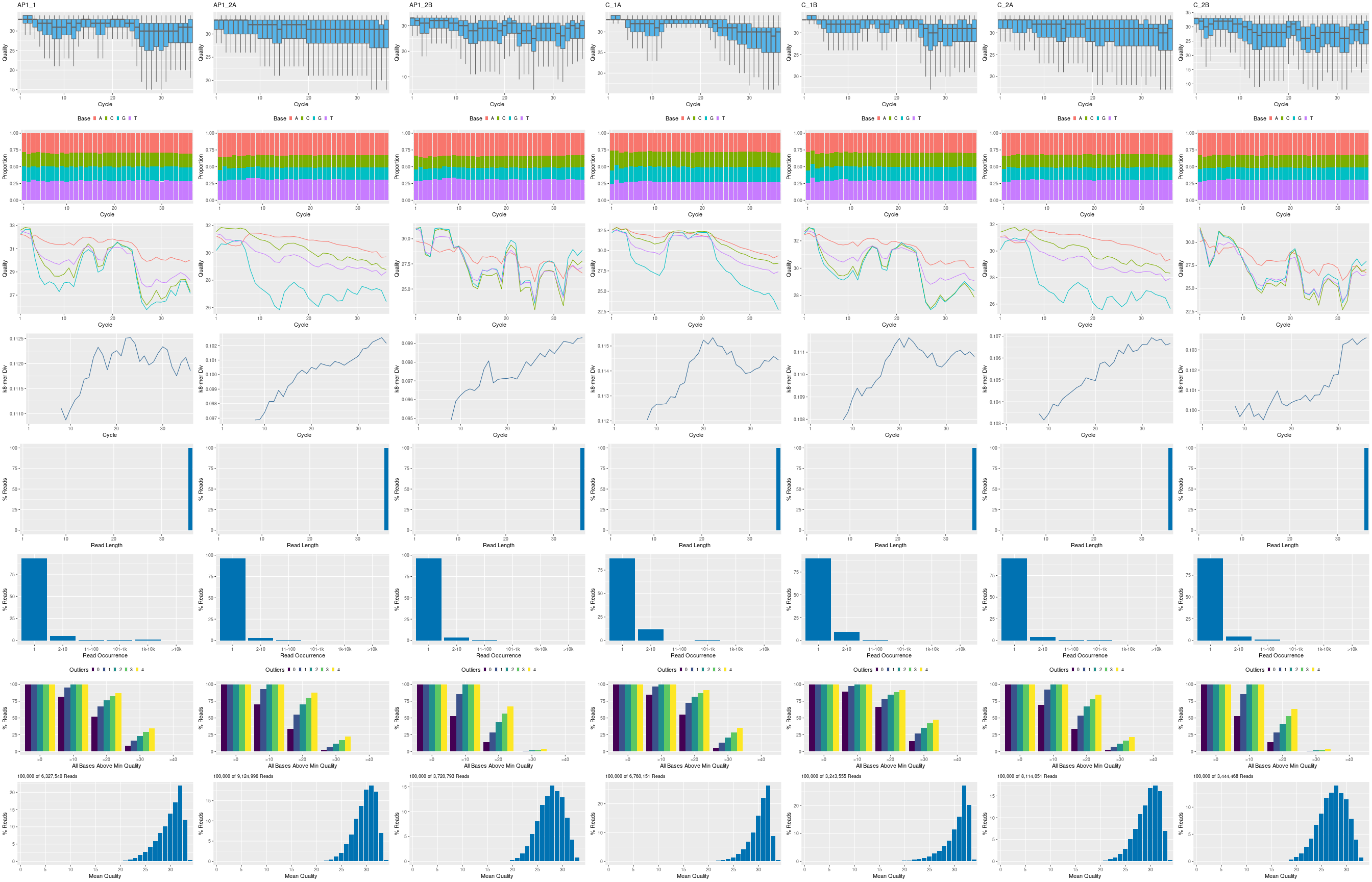
Figure 1: FASTQ quality report for 7 samples.
Alignments
Read mapping with Bowtie2
The NGS reads of this project will be aligned with Bowtie2 against the
reference genome sequence (Langmead and Salzberg 2012). The parameter settings of the
aligner are defined in the bowtie2-index.cwl and bowtie2-index.yml files.
In ChIP-Seq experiments it is usually more appropriate to eliminate reads mapping
to multiple locations. To achieve this, users want to remove the argument setting
-k 50 non-deterministic in the configuration files.
Building the index:
idx <- loadWorkflow(targets = NULL, wf_file = "bowtie2-index.cwl",
    input_file = "bowtie2-index.yml", dir_path = "param/cwl/bowtie2/bowtie2-idx")
idx <- renderWF(idx)
idx
cmdlist(idx)

## Run in single machine
runCommandline(idx, make_bam = FALSE)
The following submits 7 alignment jobs via a scheduler to a computer cluster.
targets <- "targets_chip_trim.txt"
dir_path <- "param/cwl/bowtie2/bowtie2-se"
args <- loadWF(targets = targets, wf_file = "bowtie2-mapping-se.cwl",
    input_file = "bowtie2-mapping-se.yml", dir_path = dir_path)
args <- renderWF(args, inputvars = c(FileName = "_FASTQ_PATH1_",
    SampleName = "_SampleName_"))
args
cmdlist(args)[1:2]
output(args)[1:2]
moduleload(modules(args))  # Skip if a module system is not used
resources <- list(walltime = 120, ntasks = 1, ncpus = 4, memory = 1024)
reg <- clusterRun(args, FUN = runCommandline, more.args = list(args = args,
    dir = FALSE), conffile = ".batchtools.conf.R", template = "batchtools.slurm.tmpl",
    Njobs = 7, runid = "01", resourceList = resources)
getStatus(reg = reg)
waitForJobs(reg = reg)
args <- output_update(args, dir = FALSE, replace = TRUE, extension = c(".sam",
    ".bam"))  ## Updates the output(args) to the right location in the subfolders
output(args)
Alternatively, one can run the alignments sequentially on a single system. Note: this step is not used here!
# args <- runCommandline(args, force=FALSE)
Check whether all BAM files and the corresponding new targets have been created.
writeTargetsout(x = args, file = "targets_bam.txt", step = 1,
    new_col = "FileName", new_col_output_index = 1, overwrite = TRUE,
    remove = TRUE)
outpaths <- subsetWF(args, slot = "output", subset = 1, index = 1)
file.exists(outpaths)
Read and alignment stats
The following provides an overview of the number of reads in each sample and how many of them aligned to the reference.
read_statsDF <- alignStats(args = args, output_index = 1, subset = "FileName")
write.table(read_statsDF, "results/alignStats.xls", row.names = FALSE,
    quote = FALSE, sep = "\t")
read.delim("results/alignStats.xls")
Create symbolic links for viewing BAM files in IGV
The symLink2bam function creates symbolic links to view the BAM alignment
files in a genome browser such as IGV without moving these large files to a
local system. The corresponding URLs are written to a file with a path
specified under urlfile, here IGVurl.txt. Please replace the directory
and the user name. The following parameter settings will create a
subdirectory under ~/.html called somedir of the user account. The user
name under urlbase, here ttest, needs to be changed to the corresponding
user name of the person running this function.
symLink2bam(sysargs = args, htmldir = c("~/.html/", "somedir/"),
    urlbase = "http://cluster.hpcc.ucr.edu/~<username>/", urlfile = "./results/IGVurl.txt")
Peak calling with MACS2
Merge BAM files of replicates prior to peak calling
Merging BAM files of technical and/or biological replicates can improve
the sensitivity of the peak calling by increasing the depth of read
coverage. The mergeBamByFactor function merges BAM files based on grouping information
specified by a factor, here the Factor column of the imported targets file. It
also returns an updated SYSargs2 object containing the paths to the
merged BAM files as well as to any unmerged files without replicates.
This step can be skipped if merging of BAM files is not desired.
dir_path <- "param/cwl/mergeBamByFactor"
args <- loadWF(targets = "targets_bam.txt", wf_file = "merge-bam.cwl",
    input_file = "merge-bam.yml", dir_path = dir_path)
args <- renderWF(args, inputvars = c(FileName = "_BAM_PATH_",
    SampleName = "_SampleName_"))
args_merge <- mergeBamByFactor(args = args, overwrite = TRUE)
writeTargetsout(x = args_merge, file = "targets_mergeBamByFactor.txt",
    step = 1, new_col = "FileName", new_col_output_index = 1,
    overwrite = TRUE, remove = TRUE)
Peak calling with input/reference sample
MACS2 can perform peak calling on ChIP-Seq data with and without input samples (Zhang et al. 2008).
The following performs peak calling with input sample. The input sample
can be most conveniently specified in the SampleReference column of the
initial targets file. The writeTargetsRef function uses this
information to create a targets file intermediate for running MACS2
with the corresponding input sample(s).
writeTargetsRef(infile = "targets_mergeBamByFactor.txt", outfile = "targets_bam_ref.txt",
    silent = FALSE, overwrite = TRUE)
dir_path <- "param/cwl/MACS2/MACS2-input"
args_input <- loadWF(targets = "targets_bam_ref.txt", wf_file = "macs2-input.cwl",
    input_file = "macs2.yml", dir_path = dir_path)
args_input <- renderWF(args_input, inputvars = c(FileName1 = "_FASTQ_PATH2_",
    FileName2 = "_FASTQ_PATH1_", SampleName = "_SampleName_"))
cmdlist(args_input)[1]
## Run MACS2
args_input <- runCommandline(args_input, make_bam = FALSE, force = TRUE)
outpaths_input <- subsetWF(args_input, slot = "output", subset = 1,
    index = 1)
file.exists(outpaths_input)
writeTargetsout(x = args_input, file = "targets_macs_input.txt",
    step = 1, new_col = "FileName", new_col_output_index = 1,
    overwrite = TRUE)
The peak calling results from MACS2 are written for each sample to the
results directory. They are named after the corresponding reference sample
with extensions used by MACS2.
Annotate peaks with genomic context
Annotation with ChIPseeker package
To annotate the identified peaks with genomic context information
one can use the ChIPpeakAnno or ChIPseeker package (Zhu et al. 2010; Yu, Wang, and He 2015).
The following code uses the ChIPseeker package for annotating the peaks.
library(ChIPseeker)
library(GenomicFeatures)
dir_path <- "param/cwl/annotate_peaks"
args <- loadWF(targets = "targets_macs_input.txt", wf_file = "annotate-peaks.cwl",
    input_file = "annotate-peaks.yml", dir_path = dir_path)
args <- renderWF(args, inputvars = c(FileName = "_FASTQ_PATH1_",
    SampleName = "_SampleName_"))

txdb <- makeTxDbFromGFF(file = "data/tair10.gff", format = "gff",
    dataSource = "TAIR", organism = "Arabidopsis thaliana")
for (i in seq(along = args)) {
    peakAnno <- annotatePeak(infile1(args)[i], TxDb = txdb, verbose = FALSE)
    df <- as.data.frame(peakAnno)
    outpaths <- subsetWF(args, slot = "output", subset = 1, index = 1)
    write.table(df, outpaths[i], quote = FALSE, row.names = FALSE,
        sep = "\t")
}
writeTargetsout(x = args, file = "targets_peakanno.txt", step = 1,
    new_col = "FileName", new_col_output_index = 1, overwrite = TRUE)
The peak annotation results are written to the results directory.
The files are named after the corresponding peak files with extensions
specified in the annotate_peaks.param file, here *.peaks.annotated.xls.
Count reads overlapping peaks
The countRangeset function is a convenience wrapper to perform read counting
iteratively over serveral range sets, here peak range sets. Internally,
the read counting is performed with the summarizeOverlaps function from the
GenomicAlignments package. The resulting count tables are directly saved to
files, one for each peak set.
library(GenomicRanges)
dir_path <- "param/cwl/count_rangesets"
args <- loadWF(targets = "targets_macs_input.txt", wf_file = "count_rangesets.cwl",
    input_file = "count_rangesets.yml", dir_path = dir_path)
args <- renderWF(args, inputvars = c(FileName = "_FASTQ_PATH1_",
    SampleName = "_SampleName_"))

## Bam Files
targets <- "targets_chip_trim.txt"
dir_path <- "param/cwl/bowtie2/bowtie2-se"
args_bam <- loadWF(targets = targets, wf_file = "bowtie2-mapping-se.cwl",
    input_file = "bowtie2-mapping-se.yml", dir_path = dir_path)
args_bam <- renderWF(args_bam, inputvars = c(FileName = "_FASTQ_PATH1_",
    SampleName = "_SampleName_"))
args_bam <- output_update(args_bam, dir = FALSE, replace = TRUE,
    extension = c(".sam", ".bam"))
outpaths <- subsetWF(args_bam, slot = "output", subset = 1, index = 1)

register(MulticoreParam(workers = 3))
bfl <- BamFileList(outpaths, yieldSize = 50000, index = character())
countDFnames <- countRangeset(bfl, args, mode = "Union", ignore.strand = TRUE)
writeTargetsout(x = args, file = "targets_countDF.txt", step = 1,
    new_col = "FileName", new_col_output_index = 1, overwrite = TRUE)
Shows count table generated in previous step (C_1A_peaks.countDF.xls).
To avoid slowdowns of the load time of this page, ony 200 rows of the source
table are imported into the below datatable view .
countDF <- read.delim("results/C_1A_peaks.countDF.xls")[1:200,
    ]
colnames(countDF)[1] <- "PeakIDs"
library(DT)
datatable(countDF)
Differential binding analysis
The runDiff function performs differential binding analysis in batch mode for
several count tables using edgeR or DESeq2 (Robinson, McCarthy, and Smyth 2010; Love, Huber, and Anders 2014).
Internally, it calls the functions run_edgeR and run_DESeq2. It also returns
the filtering results and plots from the downstream filterDEGs function using
the fold change and FDR cutoffs provided under the dbrfilter argument.
dir_path <- "param/cwl/rundiff"
args_diff <- loadWF(targets = "targets_countDF.txt", wf_file = "rundiff.cwl",
    input_file = "rundiff.yml", dir_path = dir_path)
args_diff <- renderWF(args_diff, inputvars = c(FileName = "_FASTQ_PATH1_",
    SampleName = "_SampleName_"))

cmp <- readComp(file = args_bam, format = "matrix")
dbrlist <- runDiff(args = args_diff, diffFct = run_edgeR, targets = targets.as.df(targets(args_bam)),
    cmp = cmp[[1]], independent = TRUE, dbrfilter = c(Fold = 2,
        FDR = 1))
writeTargetsout(x = args_diff, file = "targets_rundiff.txt",
    step = 1, new_col = "FileName", new_col_output_index = 1,
    overwrite = TRUE)
GO term enrichment analysis
The following performs GO term enrichment analysis for each annotated peak
set. Note: the following assumes that the GO annotation data exists under
data/GO/catdb.RData. If this is not the case then it can be generated with
the instructions from here.
dir_path <- "param/cwl/annotate_peaks"
args <- loadWF(targets = "targets_bam_ref.txt", wf_file = "annotate-peaks.cwl",
    input_file = "annotate-peaks.yml", dir_path = dir_path)
args <- renderWF(args, inputvars = c(FileName1 = "_FASTQ_PATH1_",
    FileName2 = "_FASTQ_PATH2_", SampleName = "_SampleName_"))

args_anno <- loadWF(targets = "targets_macs_input.txt", wf_file = "annotate-peaks.cwl",
    input_file = "annotate-peaks.yml", dir_path = dir_path)
args_anno <- renderWF(args_anno, inputvars = c(FileName = "_FASTQ_PATH1_",
    SampleName = "_SampleName_"))
annofiles <- subsetWF(args_anno, slot = "output", subset = 1,
    index = 1)
gene_ids <- sapply(names(annofiles), function(x) unique(as.character(read.delim(annofiles[x])[,
    "geneId"])), simplify = FALSE)
load("data/GO/catdb.RData")
BatchResult <- GOCluster_Report(catdb = catdb, setlist = gene_ids,
    method = "all", id_type = "gene", CLSZ = 2, cutoff = 0.9,
    gocats = c("MF", "BP", "CC"), recordSpecGO = NULL)
write.table(BatchResult, "results/GOBatchAll.xls", row.names = FALSE,
    quote = FALSE, sep = "\t")
Shows GO term enrichment results from previous step. The last gene identifier column (10)
of this table has been excluded in this viewing instance to minimze the complexity of the
result.
To avoid slowdowns of the load time of this page, ony 200 rows of the source
table are imported into the below datatable view .
BatchResult <- read.delim("results/GOBatchAll.xls")[1:200, ]
library(DT)
datatable(BatchResult[, -10], options = list(scrollX = TRUE,
    autoWidth = TRUE))
Motif analysis
Parse DNA sequences of peak regions from genome
Enrichment analysis of known DNA binding motifs or de novo discovery
of novel motifs requires the DNA sequences of the identified peak
regions. To parse the corresponding sequences from the reference genome,
the getSeq function from the Biostrings package can be used. The
following example parses the sequences for each peak set and saves the
results to separate FASTA files, one for each peak set. In addition, the
sequences in the FASTA files are ranked (sorted) by increasing p-values
as expected by some motif discovery tools, such as BCRANK.
library(Biostrings)
library(seqLogo)
library(BCRANK)
dir_path <- "param/cwl/annotate_peaks"
args <- loadWF(targets = "targets_macs_input.txt", wf_file = "annotate-peaks.cwl",
    input_file = "annotate-peaks.yml", dir_path = dir_path)
args <- renderWF(args, inputvars = c(FileName = "_FASTQ_PATH1_",
    SampleName = "_SampleName_"))

rangefiles <- infile1(args)
for (i in seq(along = rangefiles)) {
    df <- read.delim(rangefiles[i], comment = "#")
    peaks <- as(df, "GRanges")
    names(peaks) <- paste0(as.character(seqnames(peaks)), "_",
        start(peaks), "-", end(peaks))
    peaks <- peaks[order(values(peaks)$X.log10.pvalue., decreasing = TRUE)]
    pseq <- getSeq(FaFile("./data/tair10.fasta"), peaks)
    names(pseq) <- names(peaks)
    writeXStringSet(pseq, paste0(rangefiles[i], ".fasta"))
}
Motif discovery with BCRANK
The Bioconductor package BCRANK is one of the many tools available for
de novo discovery of DNA binding motifs in peak regions of ChIP-Seq
experiments. The given example applies this method on the first peak
sample set and plots the sequence logo of the highest ranking motif.
set.seed(0)
BCRANKout <- bcrank(paste0(rangefiles[1], ".fasta"), restarts = 25,
    use.P1 = TRUE, use.P2 = TRUE)
toptable(BCRANKout)
topMotif <- toptable(BCRANKout, 1)
weightMatrix <- pwm(topMotif, normalize = FALSE)
weightMatrixNormalized <- pwm(topMotif, normalize = TRUE)
png("results/seqlogo.png")
seqLogo(weightMatrixNormalized)
dev.off()
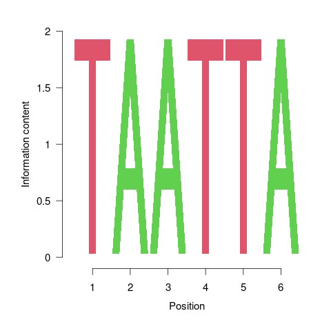
Figure 2: One of the motifs identified by BCRANK
Version Information
sessionInfo()
## R version 4.0.5 (2021-03-31)
## Platform: x86_64-pc-linux-gnu (64-bit)
## Running under: Debian GNU/Linux 10 (buster)
##
## Matrix products: default
## BLAS:   /usr/lib/x86_64-linux-gnu/blas/libblas.so.3.8.0
## LAPACK: /usr/lib/x86_64-linux-gnu/lapack/liblapack.so.3.8.0
##
## locale:
##  [1] LC_CTYPE=en_US.UTF-8       LC_NUMERIC=C
##  [3] LC_TIME=en_US.UTF-8        LC_COLLATE=en_US.UTF-8
##  [5] LC_MONETARY=en_US.UTF-8    LC_MESSAGES=en_US.UTF-8
##  [7] LC_PAPER=en_US.UTF-8       LC_NAME=C
##  [9] LC_ADDRESS=C               LC_TELEPHONE=C
## [11] LC_MEASUREMENT=en_US.UTF-8 LC_IDENTIFICATION=C
##
## attached base packages:
## [1] stats4    parallel  stats     graphics  grDevices
## [6] utils     datasets  methods   base
##
## other attached packages:
##  [1] systemPipeR_1.24.5          ShortRead_1.48.0
##  [3] GenomicAlignments_1.26.0    SummarizedExperiment_1.20.0
##  [5] Biobase_2.50.0              MatrixGenerics_1.2.0
##  [7] matrixStats_0.57.0          BiocParallel_1.24.1
##  [9] Rsamtools_2.6.0             Biostrings_2.58.0
## [11] XVector_0.30.0              GenomicRanges_1.42.0
## [13] GenomeInfoDb_1.26.1         IRanges_2.24.0
## [15] S4Vectors_0.28.0            BiocGenerics_0.36.0
## [17] BiocStyle_2.18.0
##
## loaded via a namespace (and not attached):
##   [1] colorspace_2.0-0         rjson_0.2.20
##   [3] hwriter_1.3.2            ellipsis_0.3.1
##   [5] bit64_4.0.5              AnnotationDbi_1.52.0
##   [7] xml2_1.3.2               codetools_0.2-18
##   [9] splines_4.0.5            knitr_1.30
##  [11] jsonlite_1.7.1           annotate_1.68.0
##  [13] GO.db_3.12.1             dbplyr_2.0.0
##  [15] png_0.1-7                pheatmap_1.0.12
##  [17] graph_1.68.0             BiocManager_1.30.10
##  [19] compiler_4.0.5           httr_1.4.2
##  [21] backports_1.2.0          GOstats_2.56.0
##  [23] assertthat_0.2.1         Matrix_1.3-2
##  [25] limma_3.46.0             formatR_1.7
##  [27] htmltools_0.5.1.1        prettyunits_1.1.1
##  [29] tools_4.0.5              gtable_0.3.0
##  [31] glue_1.4.2               GenomeInfoDbData_1.2.4
##  [33] Category_2.56.0          dplyr_1.0.2
##  [35] rsvg_2.1                 batchtools_0.9.14
##  [37] rappdirs_0.3.1           V8_3.4.0
##  [39] Rcpp_1.0.5               jquerylib_0.1.3
##  [41] vctrs_0.3.5              blogdown_1.2
##  [43] rtracklayer_1.50.0       xfun_0.22
##  [45] stringr_1.4.0            lifecycle_0.2.0
##  [47] XML_3.99-0.5             edgeR_3.32.0
##  [49] zlibbioc_1.36.0          scales_1.1.1
##  [51] BSgenome_1.58.0          VariantAnnotation_1.36.0
##  [53] hms_0.5.3                RBGL_1.66.0
##  [55] RColorBrewer_1.1-2       yaml_2.2.1
##  [57] curl_4.3                 memoise_1.1.0
##  [59] ggplot2_3.3.2            sass_0.3.1
##  [61] biomaRt_2.46.0           latticeExtra_0.6-29
##  [63] stringi_1.5.3            RSQLite_2.2.1
##  [65] genefilter_1.72.0        checkmate_2.0.0
##  [67] GenomicFeatures_1.42.1   DOT_0.1
##  [69] rlang_0.4.8              pkgconfig_2.0.3
##  [71] bitops_1.0-6             evaluate_0.14
##  [73] lattice_0.20-41          purrr_0.3.4
##  [75] bit_4.0.4                tidyselect_1.1.0
##  [77] GSEABase_1.52.0          AnnotationForge_1.32.0
##  [79] magrittr_2.0.1           bookdown_0.21
##  [81] R6_2.5.0                 generics_0.1.0
##  [83] base64url_1.4            DelayedArray_0.16.0
##  [85] DBI_1.1.0                withr_2.3.0
##  [87] pillar_1.4.7             survival_3.2-10
##  [89] RCurl_1.98-1.2           tibble_3.0.4
##  [91] crayon_1.3.4             BiocFileCache_1.14.0
##  [93] rmarkdown_2.7            jpeg_0.1-8.1
##  [95] progress_1.2.2           locfit_1.5-9.4
##  [97] grid_4.0.5               data.table_1.13.2
##  [99] blob_1.2.1               Rgraphviz_2.34.0
## [101] digest_0.6.27            xtable_1.8-4
## [103] brew_1.0-6               openssl_1.4.3
## [105] munsell_0.5.0            bslib_0.2.4
## [107] askpass_1.1
Funding
This project was supported by funds from the National Institutes of Health (NIH) and the National Science Foundation (NSF).
References
H Backman, Tyler W, and Thomas Girke. 2016. “systemPipeR: NGS workflow and report generation environment.” BMC Bioinformatics 17 (1): 388. https://doi.org/10.1186/s12859-016-1241-0.
Kaufmann, Kerstin, Frank Wellmer, Jose M Muiño, Thilia Ferrier, Samuel E Wuest, Vijaya Kumar, Antonio Serrano-Mislata, et al. 2010. “Orchestration of floral initiation by APETALA1.” Science 328 (5974): 85–89. https://doi.org/10.1126/science.1185244.
Langmead, Ben, and Steven L Salzberg. 2012. “Fast Gapped-Read Alignment with Bowtie 2.” Nat. Methods 9 (4): 357–59. https://doi.org/10.1038/nmeth.1923.
Love, Michael, Wolfgang Huber, and Simon Anders. 2014. “Moderated Estimation of Fold Change and Dispersion for RNA-seq Data with DESeq2.” Genome Biol. 15 (12): 550. https://doi.org/10.1186/s13059-014-0550-8.
Robinson, M D, D J McCarthy, and G K Smyth. 2010. “edgeR: A Bioconductor Package for Differential Expression Analysis of Digital Gene Expression Data.” Bioinformatics 26 (1): 139–40. https://doi.org/10.1093/bioinformatics/btp616.
Yu, Guangchuang, Li-Gen Wang, and Qing-Yu He. 2015. “ChIPseeker: An R/Bioconductor Package for ChIP Peak Annotation, Comparison and Visualization.” Bioinformatics 31 (14): 2382–83. https://doi.org/10.1093/bioinformatics/btv145.
Zhang, Y, T Liu, C A Meyer, J Eeckhoute, D S Johnson, B E Bernstein, C Nussbaum, et al. 2008. “Model-Based Analysis of ChIP-Seq (MACS).” Genome Biol. 9 (9). https://doi.org/10.1186/gb-2008-9-9-r137.
Zhu, Lihua J, Claude Gazin, Nathan D Lawson, Hervé Pagès, Simon M Lin, David S Lapointe, and Michael R Green. 2010. “ChIPpeakAnno: A Bioconductor Package to Annotate ChIP-seq and ChIP-chip Data.” BMC Bioinformatics 11: 237. https://doi.org/10.1186/1471-2105-11-237.